Raquifer
Raquifer.Rmd
Raquifer
Raquifer estimates the cumulative water influx into hydrocarbon reservoirs using un-steady and pseudo-steady state modeling approaches. It generates a data frame of cumulative water influx over time for edge-drive and bottom-drive aquifers. Van Everdingen and Hurst un-steady state model for the constant terminal pressure solution predicts the cumulative influx for edge-water drive aquifers with radial flow (Van Everdingen & Hurst, 1949). For the bottom-water drive aquifers with linear/radial flow, the Yildiz-Khosravi un-steady state model for the constant terminal pressure solution is used (Yildiz & Khosravi, 2007). Nabor and Barham linear flow model for the constant terminal pressure solution is used for the edge-water and bottom-water drive aquifers modeling(Nabor & Barham, 1964). For the linear and radial pseudo-steady state flow modeling in aquifers, the Fetkovich method is used (Fetkovich, 1971).
Cumulative water influx predictions are generated by three different functions: aquifer_param(), aquifer_time(), and aquifer_predict().
aquifer_param() arguments
-
input_unit: A unit system for parameters, a character string either ‘SI’ or ‘Field’ -
output_unit: A unit system for properties, a character string either ‘SI’ or ‘Field’ -
param model: State of flow in the aquifer, a character string either ‘uss’ for the un-steady state flow or ‘pss’ for the pseudo-steady state flow -
flow_type: A character string either ‘radial’ or ‘linear’ -
water_drive: A character string either ‘edge’ or ‘bottom’ -
phi: Aquifer porosity, a numeric fraction -
perm_h: Aquifer horizontal permeability in ‘md’ in both ‘SI’ and ‘Field’ input unit systems. A NULL value must be used for the combination of ‘uss’, ‘linear’, and ‘bottom’ flow -
perm_v: Aquifer vertical permeability in ‘md’ in both ‘SI’ and ‘Field’ input unit systems. A NULL value must be used for the combination of ‘uss’, ‘linear’, ‘edge’ flow. A NULL value must be used for the combination of ‘uss’, ‘radial’, ‘edge’ flow. A NULL value must be used for the combination of ‘pss’, ‘radial’, ‘edge’ flow. -
h_a: Aquifer` height in ‘m’ or ‘ft’ in ‘SI’ and ‘Field’ input unit systems, respectively. -
r_a: Aquifer radius in ‘m’ or ‘ft’ in ‘SI’ and ‘Field’ input unit systems, respectively. A NULL value must be used for the combination of ‘uss’, ‘linear’, ‘edge’ flow. A NULL value must be used for the combination of ‘uss’, ‘linear’, ‘bottom’ flow. -
r_R: Reservoir radius in ‘m’ or ‘ft’ in ‘SI’ and ‘Field’ input unit systems, respectively. A NULL value must be used for the combination of ‘uss’, ‘linear’, ‘edge’ flow. A NULL value must be used for the combination of ‘uss’, ‘linear’, ‘bottom’ flow. -
w_a: Aquifer width in ‘m’ or ‘ft’ in ‘SI’ and ‘Field’ input unit systems, respectively. A NULL value must be used for the combination of ‘uss’, ‘radial’, ‘edge’ flow. A NULL value must be used for the combination of ‘uss’, ‘radial’, ‘bottom’ flow. A NULL value must be used for the combination of ‘pss’, ‘radial’, ‘edge’ flow. -
l_a: Aquifer length in ‘m’ or ‘ft’ in ‘SI’ and ‘Field’ input unit systems, respectively. A NULL value must be used for the combination of ‘uss’, ‘radial’, ‘edge’ flow. A NULL value must be used for the combination of ‘uss’, ‘radial’, ‘bottom’ flow. A NULL value must be used for the combination of ‘pss’, ‘radial’, ‘edge’ flow. -
tetha: Fraction of reservoir encircled by the aquifer, reported in “degrees” in both ‘SI’ and ‘Field’ input unit systems. A NULL value must be used for the combination of ‘uss’, ‘radial’, ‘bottom’ flow. A NULL value must be used for the combination of ‘uss’, ‘linear’, ‘edge’ flow. A NULL value must be used for the combination of ‘uss’, ‘linear’, ‘bottom’ flow. -
mu_water: Water viscosity in ‘mPa.s’ or ‘cp’ in ‘SI’ and ‘Field’ input unit systems, respectively -
c_water: Water compressibility in ‘1/kPa’ or ‘1/psi’ in ‘SI’ and ‘Field’ input unit systems, respectively -
c_rock: Rock compressibility in ‘1/kPa’ or ‘1/psi’ in ‘SI’ and ‘Field’ input unit systems, respectively -
pressure: A numeric vector of pressure data at the boundary of reservoir/aquifer. Must have the same length as the ‘aquifer_time()’ object
aquifer_time() arguments
-
x: A vector or sequence of times/dates. -
unit: A unit system for input vector x.
aquifer_predict() arguments
-
aquifer_lst: A list object of class ‘decline’. -
time_lst: A list object of class ‘time’
Examples
Example 1: Un-steady state radial flow, edge-water drive
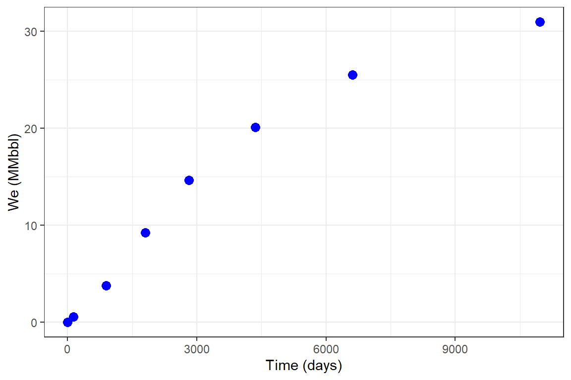
library(Raquifer)
library(ggplot2)
library(magrittr)

aqu_time <- aquifer_time(x = c(0,0.368,2.439,4.957,7.732,11.926,18.126,30.044) * 365, unit = "day")

parameters <- aquifer_param(input_unit = "Field", output_unit = "Field", model = "uss",
                            flow_type = "radial", water_drive = "edge", phi = 0.27, perm_h = 64.2,
                            h_a = 20, r_a = 5 * 14892, r_R = 14892, tetha = 180,
                            mu_water = 0.485, c_water = 3.88e-6, c_rock = 2e-6,
                            pressure = c(1640,1600,1400,1200,1000,800,600,400))

aqu_time
#> $t
#> [1]     0.000   134.320   890.235  1809.305  2822.180  4352.990  6615.990
#> [8] 10966.060
#>
#> $unit
#> [1] "day"
#>
#> $reference_date
#> [1] "2020-07-04"
#>
#> attr(,"class")
#> [1] "day"  "time"

parameters
#> $input_unit
#> [1] "Field"
#>
#> $output_unit
#> [1] "Field"
#>
#> $model
#> [1] "veh_rad_edge"
#>
#> $phi
#> [1] 0.27
#>
#> $perm_h
#> [1] 64.2
#>
#> $h_a
#> [1] 20
#>
#> $r_a
#> [1] 74460
#>
#> $r_R
#> [1] 14892
#>
#> $tetha
#> [1] 180
#>
#> $mu_water
#> [1] 0.485
#>
#> $c_water
#> [1] 3.88e-06
#>
#> $c_rock
#> [1] 2e-06
#>
#> $pressure
#> [1] 1640 1600 1400 1200 1000  800  600  400
#>
#> attr(,"class")
#> [1] "veh_rad_edge" "aquifer"

pred_veh <- aquifer_predict(aquifer_lst = parameters, time_lst = aqu_time)

head(pred_veh)
#>         Date Time (days)  We (MMbbl)
#> 1 2020-07-04       0.000  0.00000000
#> 2 2020-11-15     134.320  0.06185335
#> 3 2022-12-11     890.235  1.27831951
#> 4 2025-06-17    1809.305  4.19222802
#> 5 2028-03-26    2822.180  8.46586625
#> 6 2032-06-03    4352.990 15.65627937

pred_veh %>% ggplot(aes(x = `Time (days)`, y = `We (MMbbl)`)) +
  geom_point(size = 3, color = "blue") +
  theme_bw()

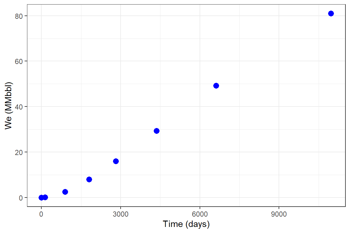
Example 2: Un-steady state radial flow, bottom-water drive
library(Raquifer)
library(ggplot2)
library(magrittr)

aqu_time <- aquifer_time(x = c(0,0.368,2.439,4.957,7.732,11.926,18.126,30.044) * 365, unit = "day")

parameters <- aquifer_param(input_unit = "Field", output_unit = "Field", model = "uss",
                            flow_type = "radial", water_drive = "bottom", phi = 0.27, perm_h = 64.2,
                            perm_v = 64.2, h_a = 20, r_a = 5 * 14892, r_R = 14892,
                            mu_water = 0.485, c_water = 3.88e-6, c_rock = 2e-6,
                            pressure = c(1640,1600,1400,1200,1000,800,600,400))

pred_ykh <- aquifer_predict(aquifer_lst = parameters, time_lst = aqu_time)

head(pred_ykh)
#>         Date Time (days) We (MMbbl)
#> 1 2020-07-04       0.000  0.0000000
#> 2 2020-11-15     134.320  0.1600501
#> 3 2022-12-11     890.235  2.5380986
#> 4 2025-06-17    1809.305  8.0646132
#> 5 2028-03-26    2822.180 16.0265710
#> 6 2032-06-03    4352.990 29.3508862

pred_ykh %>% ggplot(aes(x = `Time (days)`, y = `We (MMbbl)`)) +
  geom_point(size = 3, color = "blue") +
  theme_bw()
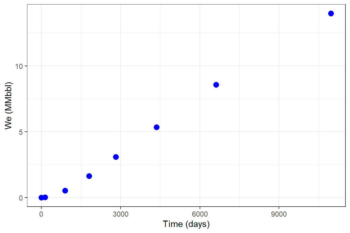
Example 3: Pseudo-steady state radial flow, edge-water drive
library(Raquifer)
library(ggplot2)
library(magrittr)

aqu_time <- aquifer_time(x = c(0,0.368,2.439,4.957,7.732,11.926,18.126,30.044) * 365, unit = "day")

parameters <- aquifer_param(input_unit = "Field", output_unit = "Field", model = "pss",
                            flow_type = "radial", water_drive = "edge", phi = 0.27, perm_h = 64.2,
                            h_a = 20, r_a = 5 * 14892, r_R = 14892, tetha = 180,
                            mu_water = 0.485, c_water = 3.88e-6, c_rock = 2e-6,
                            pressure = c(1640,1600,1400,1200,1000,800,600,400))

pred_fetk <- aquifer_predict(aquifer_lst = parameters, time_lst = aqu_time)

head(pred_fetk)
#>         Date Time (days)  We (MMbbl)
#> 1 2020-07-04       0.000  0.00000000
#> 2 2020-11-15     134.320  0.02884514
#> 3 2022-12-11     890.235  1.08324703
#> 4 2025-06-17    1809.305  3.94690549
#> 5 2028-03-26    2822.180  8.44348341
#> 6 2032-06-03    4352.990 16.33925334

pred_fetk %>% ggplot(aes(x = `Time (days)`, y = `We (MMbbl)`)) +
  geom_point(size = 3, color = "blue") +
  theme_bw()
Example 4: Un-steady state linear flow, edge-water drive
library(Raquifer)
library(ggplot2)
library(magrittr)

aqu_time <- aquifer_time(x = c(0,0.368,2.439,4.957,7.732,11.926,18.126,30.044) * 365, unit = "day")

parameters <- aquifer_param(input_unit = "Field", output_unit = "Field", model = "uss",
                            flow_type = "linear", water_drive = "edge", phi = 0.27, perm_h = 64.2,
                            h_a = 20, w_a = 29784, l_a = 161145, mu_water = 0.485, c_water = 3.88e-6,
                            c_rock = 2e-6, pressure = c(1640,1600,1400,1200,1000,800,600,400))

pred_nb_01 <- aquifer_predict(aquifer_lst = parameters, time_lst = aqu_time)

head(pred_nb_01)
#>         Date Time (days) We (MMbbl)
#> 1 2020-07-04       0.000 0.00000000
#> 2 2020-11-15     134.320 0.03199772
#> 3 2022-12-11     890.235 0.53782163
#> 4 2025-06-17    1809.305 1.63239439
#> 5 2028-03-26    2822.180 3.09768169
#> 6 2032-06-03    4352.990 5.35540873

pred_nb_01 %>% ggplot(aes(x = `Time (days)`, y = `We (MMbbl)`)) +
  geom_point(size = 3, color = "blue") +
  theme_bw()
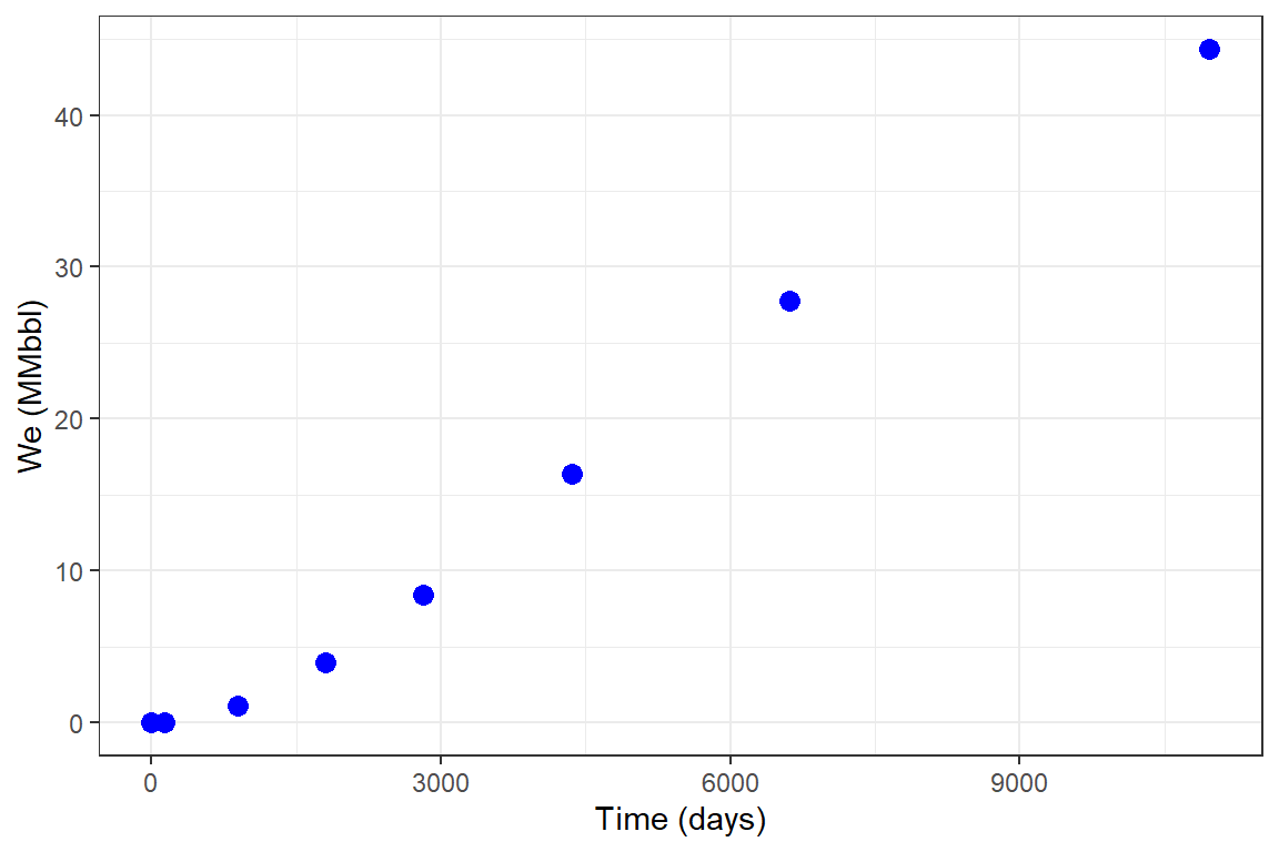
Example 5: Un-steady state linear flow, bottom-water drive
library(Raquifer)
library(ggplot2)
library(magrittr)

aqu_time <- aquifer_time(x = c(0,0.368,2.439,4.957,7.732,11.926,18.126,30.044) * 365, unit = "day")

parameters <- aquifer_param(input_unit = "Field", output_unit = "Field", model = "uss",
                            flow_type = "linear", water_drive = "bottom", phi = 0.27, perm_v = 64.2,
                            h_a = 20, w_a = 29784, l_a = 161145, mu_water = 0.485, c_water = 3.88e-6,
                            c_rock = 2e-6, pressure = c(1640,1600,1400,1200,1000,800,600,400))

pred_nb_02 <- aquifer_predict(aquifer_lst = parameters, time_lst = aqu_time)

head(pred_nb_02)
#>         Date Time (days) We (MMbbl)
#> 1 2020-07-04       0.000  0.0000000
#> 2 2020-11-15     134.320  0.5428142
#> 3 2022-12-11     890.235  3.7996992
#> 4 2025-06-17    1809.305  9.2278409
#> 5 2028-03-26    2822.180 14.6559827
#> 6 2032-06-03    4352.990 20.0841244

pred_nb_02 %>% ggplot(aes(x = `Time (days)`, y = `We (MMbbl)`)) +
  geom_point(size = 3, color = "blue") +
  theme_bw()

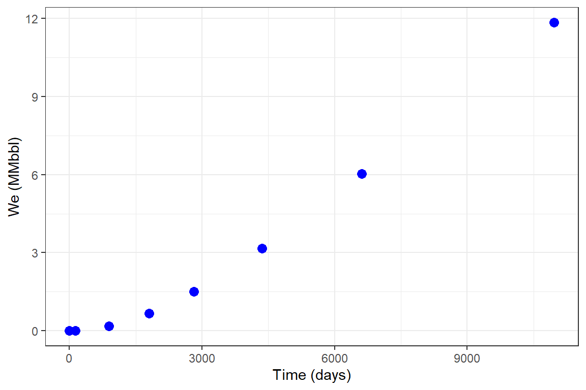
Example 6: Pseudo-steady state linear flow, edge-water drive
library(Raquifer)
library(ggplot2)
library(magrittr)

aqu_time <- aquifer_time(x = c(0,0.368,2.439,4.957,7.732,11.926,18.126,30.044) * 365, unit = "day")

parameters <- aquifer_param(input_unit = "Field", output_unit = "Field", model = "pss",
                            flow_type = "linear", water_drive = "edge", phi = 0.27, perm_h = 64.2,
                            h_a = 20, w_a = 29784, l_a = 161145, mu_water = 0.485, c_water = 3.88e-6,
                            c_rock = 2e-6, pressure = c(1640,1600,1400,1200,1000,800,600,400))

parameters
#> $input_unit
#> [1] "Field"
#>
#> $output_unit
#> [1] "Field"
#>
#> $model
#> [1] "fetk_lin_edge"
#>
#> $phi
#> [1] 0.27
#>
#> $perm_h
#> [1] 64.2
#>
#> $h_a
#> [1] 20
#>
#> $w_a
#> [1] 29784
#>
#> $l_a
#> [1] 161145
#>
#> $mu_water
#> [1] 0.485
#>
#> $c_water
#> [1] 3.88e-06
#>
#> $c_rock
#> [1] 2e-06
#>
#> $pressure
#> [1] 1640 1600 1400 1200 1000  800  600  400
#>
#> attr(,"class")
#> [1] "fetk_lin_edge" "aquifer"

pred_fetk_02 <- aquifer_predict(aquifer_lst = parameters, time_lst = aqu_time)

head(pred_fetk_02)
#>         Date Time (days)  We (MMbbl)
#> 1 2020-07-04       0.000 0.000000000
#> 2 2020-11-15     134.320 0.004426176
#> 3 2022-12-11     890.235 0.175334148
#> 4 2025-06-17    1809.305 0.668533598
#> 5 2028-03-26    2822.180 1.506005132
#> 6 2032-06-03    4352.990 3.161133684

pred_fetk_02 %>% ggplot(aes(x = `Time (days)`, y = `We (MMbbl)`)) +
  geom_point(size = 3, color = "blue") +
  theme_bw()
Example 7: Pseudo-steady state linear flow, bottom-water drive
library(Raquifer)
library(ggplot2)
library(magrittr)

aqu_time <- aquifer_time(x = c(0,0.368,2.439,4.957,7.732,11.926,18.126,30.044) * 365, unit = "day")

parameters <- aquifer_param(input_unit = "Field", output_unit = "Field", model = "pss",
                            flow_type = "linear", water_drive = "bottom", phi = 0.27, perm_v = 64.2,
                            h_a = 20, w_a = 29784, l_a = 161145, mu_water = 0.485, c_water = 3.88e-6,
                            c_rock = 2e-6, pressure = c(1640,1600,1400,1200,1000,800,600,400))

pred_fetk_03 <- aquifer_predict(aquifer_lst = parameters, time_lst = aqu_time)

head(pred_fetk_03)
#>         Date Time (days) We (MMbbl)
#> 1 2020-07-04       0.000  0.0000000
#> 2 2020-11-15     134.320  0.5428142
#> 3 2022-12-11     890.235  3.7996992
#> 4 2025-06-17    1809.305  9.2278409
#> 5 2028-03-26    2822.180 14.6559827
#> 6 2032-06-03    4352.990 20.0841244

pred_fetk_03 %>% ggplot(aes(x = `Time (days)`, y = `We (MMbbl)`)) +
  geom_point(size = 3, color = "blue") +
  theme_bw()
Example 8: Un-steady state radial flow, edge-water drive
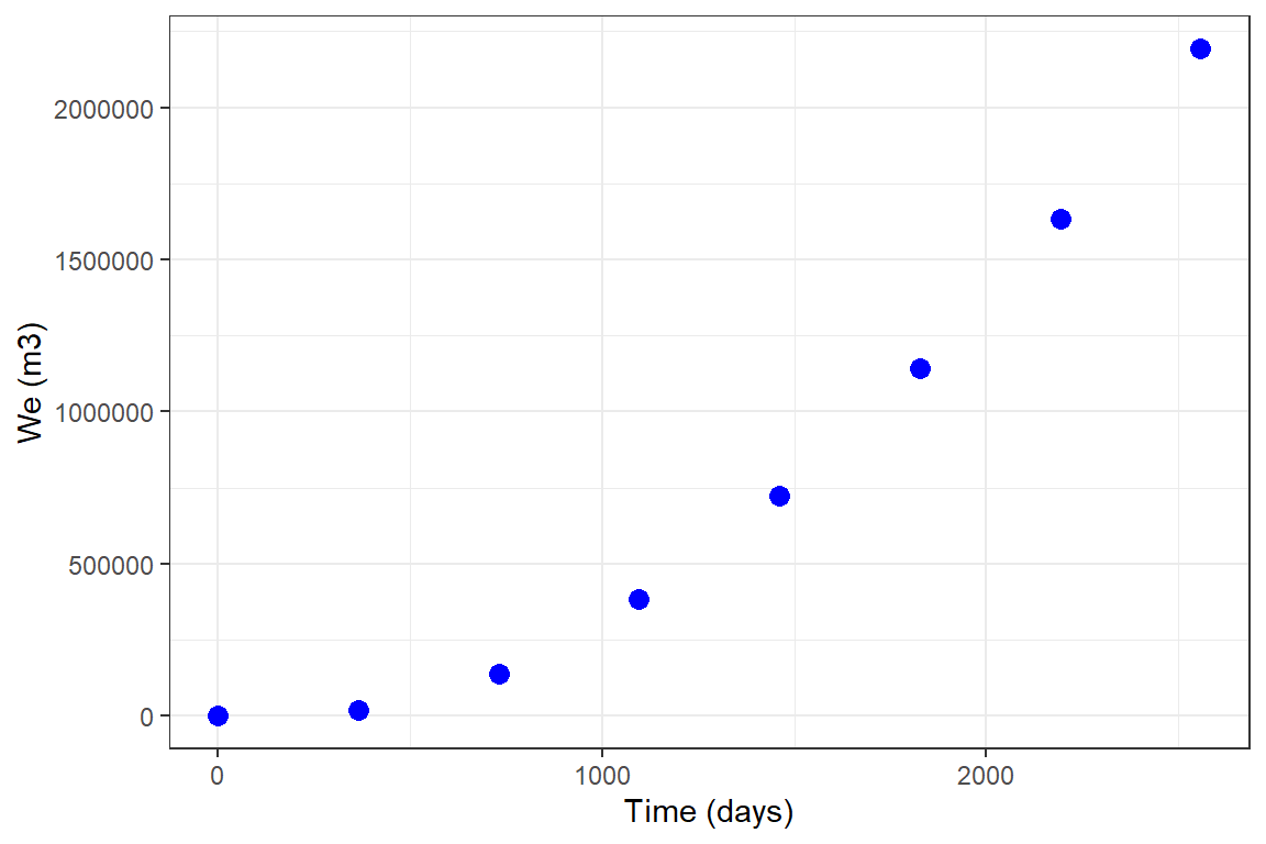
library(Raquifer)
library(ggplot2)
library(magrittr)

aqu_time <- aquifer_time(x = seq(as.Date("2020/1/1"), by = "year", length.out = 8), unit = "date")

parameters <- aquifer_param(input_unit = "Field", output_unit = "SI", model = "uss",
                            flow_type = "radial", water_drive = "edge", phi = 0.27, perm_h = 64.2,
                            h_a = 20, r_a = 5 * 14892, r_R = 14892, tetha = 180,
                            mu_water = 0.485, c_water = 3.88e-6, c_rock = 2e-6,
                            pressure = c(1640,1600,1400,1200,1000,800,600,400))

aqu_time
#> $t
#> [1]    0  366  731 1096 1461 1827 2192 2557
#>
#> $unit
#> [1] "date"
#>
#> $reference_date
#> [1] "2020-01-01"
#>
#> attr(,"class")
#> [1] "day"  "time"

parameters
#> $input_unit
#> [1] "Field"
#>
#> $output_unit
#> [1] "SI"
#>
#> $model
#> [1] "veh_rad_edge"
#>
#> $phi
#> [1] 0.27
#>
#> $perm_h
#> [1] 64.2
#>
#> $h_a
#> [1] 20
#>
#> $r_a
#> [1] 74460
#>
#> $r_R
#> [1] 14892
#>
#> $tetha
#> [1] 180
#>
#> $mu_water
#> [1] 0.485
#>
#> $c_water
#> [1] 3.88e-06
#>
#> $c_rock
#> [1] 2e-06
#>
#> $pressure
#> [1] 1640 1600 1400 1200 1000  800  600  400
#>
#> attr(,"class")
#> [1] "veh_rad_edge" "aquifer"

pred_veh <- aquifer_predict(aquifer_lst = parameters, time_lst = aqu_time)

head(pred_veh)
#>         Date Time (days)   We (m3)
#> 1 2020-01-01           0       0.0
#> 2 2021-01-01         366   18021.0
#> 3 2022-01-01         731  135900.7
#> 4 2023-01-01        1096  383984.4
#> 5 2024-01-01        1461  722190.1
#> 6 2025-01-01        1827 1141218.1

pred_veh %>% ggplot(aes(x = `Time (days)`, y = `We (m3)`)) +
  geom_point(size = 3, color = "blue") +
  theme_bw()
Example 8: Un-steady state radial flow, edge-water drive
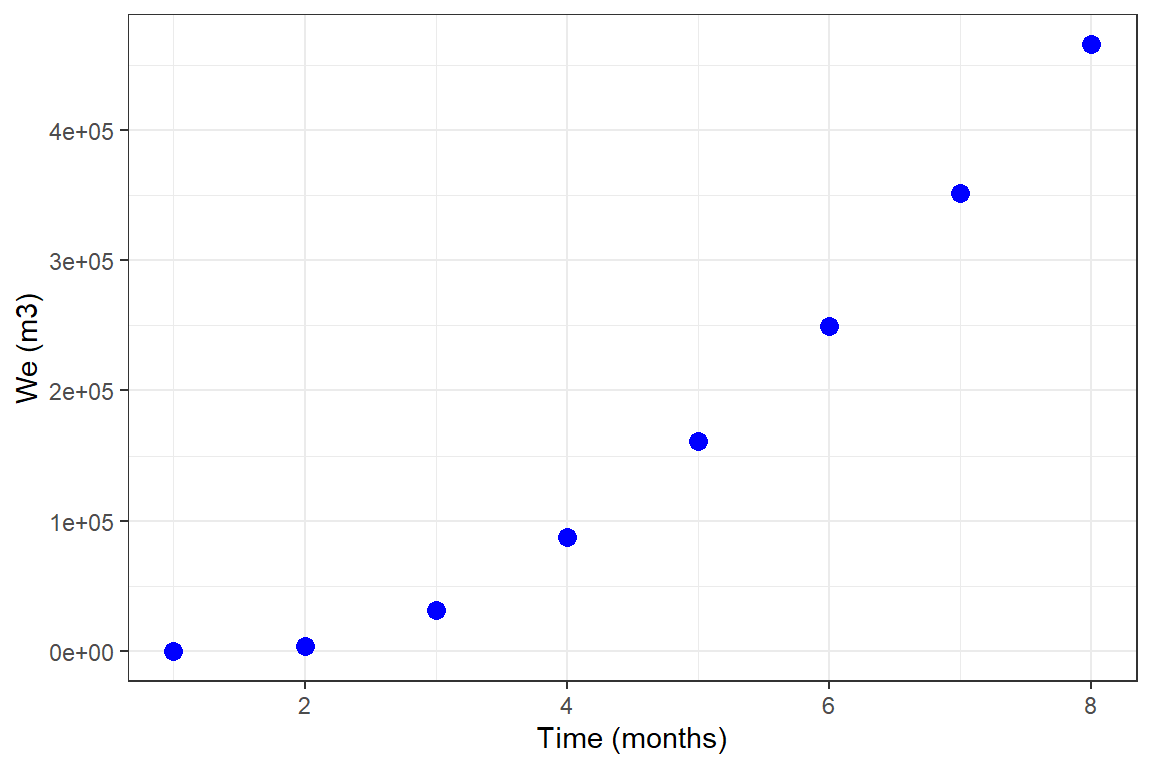
library(Raquifer)
library(ggplot2)
library(magrittr)

aqu_time <- aquifer_time(x = 1:8, unit = "month")

parameters <- aquifer_param(input_unit = "Field", output_unit = "SI", model = "uss",
                            flow_type = "radial", water_drive = "edge", phi = 0.27, perm_h = 64.2,
                            h_a = 20, r_a = 5 * 14892, r_R = 14892, tetha = 180,
                            mu_water = 0.485, c_water = 3.88e-6, c_rock = 2e-6,
                            pressure = c(1640,1600,1400,1200,1000,800,600,400))

aqu_time
#> $t
#> [1] 1 2 3 4 5 6 7 8
#>
#> $unit
#> [1] "month"
#>
#> $reference_date
#> [1] "2020-07-04"
#>
#> attr(,"class")
#> [1] "month" "time"

parameters
#> $input_unit
#> [1] "Field"
#>
#> $output_unit
#> [1] "SI"
#>
#> $model
#> [1] "veh_rad_edge"
#>
#> $phi
#> [1] 0.27
#>
#> $perm_h
#> [1] 64.2
#>
#> $h_a
#> [1] 20
#>
#> $r_a
#> [1] 74460
#>
#> $r_R
#> [1] 14892
#>
#> $tetha
#> [1] 180
#>
#> $mu_water
#> [1] 0.485
#>
#> $c_water
#> [1] 3.88e-06
#>
#> $c_rock
#> [1] 2e-06
#>
#> $pressure
#> [1] 1640 1600 1400 1200 1000  800  600  400
#>
#> attr(,"class")
#> [1] "veh_rad_edge" "aquifer"

pred_veh <- aquifer_predict(aquifer_lst = parameters, time_lst = aqu_time)

head(pred_veh)
#>         Date Time (months)    We (m3)
#> 1 2020-08-03             1      0.000
#> 2 2020-09-02             2   4236.423
#> 3 2020-10-03             3  31650.466
#> 4 2020-11-02             4  87609.327
#> 5 2020-12-03             5 161084.687
#> 6 2021-01-02             6 249479.619

pred_veh %>% ggplot(aes(x = `Time (months)`, y = `We (m3)`)) +
  geom_point(size = 3, color = "blue") +
  theme_bw()
References
Fetkovich, M. J. (1971). A Simplified Approach to Water Influx Calculations-Finite Aquifer Systems. Journal of Petroleum Technology, 23(07), 814–828. https://doi.org/10.2118/2603-PA
Nabor, G. W., & Barham, R. H. (1964). Linear Aquifer Behavior. Journal of Petroleum Technology, 16(05), 561–563. https://doi.org/10.2118/791-PA
Van Everdingen, A. F., & Hurst, W. (1949). The Application of the Laplace Transformation to Flow Problems in Reservoirs. Journal of Petroleum Technology, 1(12), 305–324. https://doi.org/10.2118/949305-G
Yildiz, T., & Khosravi, A. (2007). An Analytical Bottomwaterdrive Aquifer Model for Material-Balance Analysis. SPE Reservoir Evaluation & Engineering, 10(06), 618–628. https://doi.org/10.2118/103283-PA