Rpvt Package
Rpvt.Rmd
Rpvt
Rpvt is a correlation-based PVT (Pressure-Volume-Temperature) package for dry gas, wet gas, black oil, and water samples. It generates PVT properties of hydrocarbons and water samples in a tabular format at a constant temperature from atmospheric pressure up to the pressure of interest. Predictions for gas, oil, and water samples are generated by pvt_gas(), pvt_oil(), and pvt_water() functions, respectively.
pvt_gas() arguments
-
input_unit: input unit system for parameters, a character string either ‘SI’ or ‘Field’. -
output_unit: output unit system for properties, a character string either ‘SI’ or ‘Field’. -
fluid: fluid type, a character string either ‘dry_gas’ or ‘wet_gas’. -
pvt_model: PVT model, the character string ‘DAK’. -
visc_model: viscosity model, the character string ‘Sutton’. -
t: Reservoir temperature, a numeric value either in ‘C’ or ‘F’ depending on the ‘input_unit’. -
p: Reservoir pressure, a numeric value either in ‘kPag’ or ‘Psig’ depending on the ‘input_unit’. -
gas_spgr: gas specific gravity (Air = 1.0). -
nhc_composition: a vector of mole fractions for nitrogen, hydrogen sulfide, and carbon dioxide, respectively. -
cgr: condensate to gas ratio, a numeric value in ‘m3/m3’ or ‘STB/MMSCF’ depending on the ‘input_unit’. -
cond_api: condensate API gravity used for wet gas samples. It must beNULLfor dry gas mixtures. -
warning: a charater string either ‘yes’ or ‘no’. It shows warning messages for input parameters outside the range of correlations.
pvt_oil() arguments
-
input_unit: input_unit input unit system for parameters, a character string either ‘SI’ or ‘Field’. -
output_unit: output_unit output unit system for properties, a character string either ‘SI’ or ‘Field’. -
fluid: fluid type, the character string ‘black_oil’. -
pvt_model: PVT model, a character string. ‘Standing’, ‘Vasquez_Beggs’, ‘Farshad_Petrosky’, ‘Al_Marhoun’, and ‘Glaso’ models are currently available. -
visc_model: viscosity model, a character string. ‘Beggs_Robinson’, and ‘Al_Marhoun’ models are currently available. -
t: Reservoir temperature, a numeric value either in ‘C’ or ‘F’ depending on the ‘input_unit’. -
p: Reservoir pressure, a numeric value either in ‘kPag’ or ‘Psig’ depending on the ‘input_unit’. -
oil_api: API gravity of oil. -
gas_spgr: gas specific gravity (Air = 1.0). -
nhc_composition: a vector of mole fractions for nitrogen, hydrogen sulfide, and carbon dioxide, respectively. -
rsi: initial solution gas oil ratio in ‘m3/m3’ or ‘SCF/STB’ depending on the ‘input_unit’. It is either NULL or a numeric value. If ‘rsi’ is NULL, then a numeric value must be assigned to ‘pb’. -
pb: bubble point pressure, a numeric value either in ‘kPag’ or ‘Psig’ depending on the ‘input_unit’. it is either NULL or a numeric value. If ‘pb’ is NULL, then a numeric value must be assigned to ‘rsi’. -
warning: a charater string either ‘yes’ or ‘no’. It shows warning messages for input parameters outside the range of correlations.
pvt_water() arguments
-
input_unit: input_unit input unit system for parameters, a character string either ‘SI’ or ‘Field’. -
output_unit: output unit system for properties, a character string either ‘SI’ or ‘Field’. -
fluid: fluid type, the character string ‘water’. -
pvt_model: PVT model, a character string. ‘Spivey’, ‘Meehan’, and ‘McCain’ models are currently available. -
visc_model: viscosity model, a character string. ‘Spivey’, ‘Meehan’, and ‘McCain’ models are currently available. -
t: Reservoir temperature, a numeric value either in ‘C’ or ‘F’ depending on the ‘input_unit’. -
p: Reservoir pressure, a numeric value either in ‘kPag’ or ‘Psig’ depending on the ‘input_unit’. -
gas_saturated: a charater string either ‘yes’ or ‘no’. -
salinity: water salinity in weight percent TDS. -
warning: a charater string either ‘yes’ or ‘no’. It shows warning messages for input parameters outside the range of correlations.
Units for input parameters
The input_unit is either SI or Field. Depending on the input_unit system, the following units are used for the input parameters:
-
t: “F” in “Field” or “C” in “SI”. -
p: “Psig” in “Field” or “kPag” in “SI”. -
cgr: “STB/MMSCF” in “Field” or “m3/m3” in “SI”. -
rsi: “SCF/STB” in “Field” or “m3/m3” in “SI”. -
pb: “Psig” in “Field” or “kPag” in “SI”.
Gas Correlations
-
pvt_model: “DAK” correlation (Dranchuk and Abou-Kassem) (Sutton, 2007). -
visc_model: “Sutton” correlation (Sutton, 2007).
Oil Correlations
-
pvt_model: “Standing”, “Vasquez_Beggs”, “Farshad_Petrosky”, “Al_Marhoun”, or “Glaso” correlations (Al-Marhoun, 1988; Glaso, 1980; Petrosky Jr. & Farshad, 1998; Standing, 1947; Vasquez & Beggs, 1980). “Spivey” correlation is used for estimating the oil compressibility above the bubble point (Spivey, Valko, & McCain, 2007). -
visc_model: “Beggs_Robinson”, or “Al_Marhoun” correlations (Al-Marhoun, 2004; Beggs & Robinson, 1975).
Water Correlations
-
pvt_model: “Spivey”, “McCain” or “Meehan” correlations (McCain, Jr., Spivey, & Lenn, 2011; McCain Jr., 1991; Meehan, 1980b, 1980a; Spivey, McCain, & North, 2004). -
visc_model: “Spivey”, “McCain” or “Meehan” correlations (McCain, Jr. et al., 2011; McCain Jr., 1991; Meehan, 1980b, 1980a; Spivey et al., 2004).
Gas PVT Examples
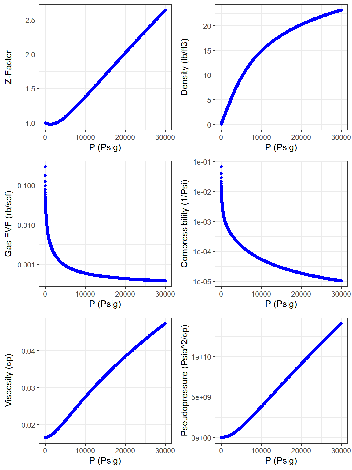
Example 1:
library(Rpvt)
library(ggplot2)
library(magrittr)
library(ggpubr)

pvt_gas_1 <- pvt_gas(input_unit = "Field", output_unit = "Field",
fluid = "dry_gas", pvt_model = "DAK", visc_model = "Sutton",
t = 400, p = 30000, gas_spgr = 0.65, nhc_composition = c(0.03,0.012,0.018),
cgr = 0, cond_api = NULL, warning = "yes")
#> Warning in pvt_gas(input_unit = "Field", output_unit = "Field", fluid =
#> "dry_gas", : pressure is greater than dry gas PVT correlation upper limit: 10000
#> psig
#> Warning in pvt_gas(input_unit = "Field", output_unit = "Field", fluid =
#> "dry_gas", : pressure is greater than gas viscosity correlation upper limit:
#> 20000 psig

attributes(pvt_gas_1)
#> $dim
#> [1] 3001    8
#>
#> $dimnames
#> $dimnames[[1]]
#> NULL
#>
#> $dimnames[[2]]
#> [1] "T_(F)"             "P_(Psig)"          "Z-Factor"
#> [4] "Bg_(rb/scf)"       "Density_(lb/cuft)" "Cg_(1/Psia)"
#> [7] "Viscosity_(cp)"    "m(p)_(Psia^2/cp)"
#>
#>
#> $`gas pseudocritical temperature (F)`
#> [1] -102.2183
#>
#> $`gas pseudocritical pressure (Psia)`
#> [1] 648.5108

pvt_gas_1 <- as.data.frame(pvt_gas_1)

head(pvt_gas_1,10)
#>    T_(F) P_(Psig)  Z-Factor Bg_(rb/scf) Density_(lb/cuft) Cg_(1/Psia)
#> 1    400        0 0.9996026  0.29449758        0.03000184 0.068072651
#> 2    400       10 0.9993343  0.17520145        0.05043034 0.040519143
#> 3    400       20 0.9990678  0.12467204        0.07086968 0.028848352
#> 4    400       30 0.9988031  0.09675307        0.09131977 0.022399782
#> 5    400       40 0.9985402  0.07904301        0.11178051 0.018309117
#> 6    400       50 0.9982790  0.06680793        0.13225179 0.015482979
#> 7    400       60 0.9980196  0.05784892        0.15273351 0.013413498
#> 8    400       70 0.9977620  0.05100557        0.17322557 0.011832661
#> 9    400       80 0.9975062  0.04560763        0.19372786 0.010585663
#> 10   400       90 0.9972522  0.04124093        0.21424029 0.009576844
#>    Viscosity_(cp) m(p)_(Psia^2/cp)
#> 1      0.01652119             0.00
#> 2      0.01652162         23856.42
#> 3      0.01652218         59833.30
#> 4      0.01652286        107935.97
#> 5      0.01652364        168169.44
#> 6      0.01652452        240538.49
#> 7      0.01652550        325047.64
#> 8      0.01652656        421701.16
#> 9      0.01652770        530503.09
#> 10     0.01652893        651457.25

colnames(pvt_gas_1) <- c("T(F)", "P(Psig)", "Z-FACTOR", "Bg(rb/scf)",
                         "Density(lb/ft3)", "Cg(1/Psi)", "MUg(cp)",
                         "m(p)(Psia^2/cp)")
Z_plot <- pvt_gas_1 %>% ggplot(aes(x = `P(Psig)`, y = `Z-FACTOR`)) +
  geom_point(color = "blue") +
  xlab(label = "P (Psig)") +
  ylab(label = "Z-Factor") +
  theme_bw()
Density_plot <- pvt_gas_1 %>% ggplot(aes(x = `P(Psig)`, y = `Density(lb/ft3)`)) +
  geom_point(color = "blue") +
  xlab(label = "P (Psig)") +
  ylab(label = "Density (lb/ft3)") +
  theme_bw()
Bg_plot <- pvt_gas_1 %>% ggplot(aes(x = `P(Psig)`, y = `Bg(rb/scf)`)) +
  geom_point(color = "blue") +
  scale_y_log10() +
  xlab(label = "P (Psig)") +
  ylab(label = "Gas FVF (rb/scf)") +
  theme_bw()
Cg_plot <- pvt_gas_1 %>% ggplot(aes(x = `P(Psig)`, y = `Cg(1/Psi)`)) +
  geom_point(color = "blue") +
  scale_y_log10() +
  xlab(label = "P (Psig)") +
  ylab(label = "Compressibility (1/Psi)") +
  theme_bw()
MUg_plot <- pvt_gas_1 %>% ggplot(aes(x = `P(Psig)`, y = `MUg(cp)`)) +
  geom_point(color = "blue") +
  xlab(label = "P (Psig)") +
  ylab(label = "Viscosity (cp)") +
  theme_bw()
mp_plot <- pvt_gas_1 %>% ggplot(aes(x = `P(Psig)`, y = `m(p)(Psia^2/cp)`)) +
  geom_point(color = "blue") +
  xlab(label = "P (Psig)") +
  ylab(label = "Pseudopressure (Psia^2/cp)") +
  theme_bw()

gas_pvt_plots <- ggarrange(Z_plot, Density_plot, Bg_plot, Cg_plot, MUg_plot, mp_plot,
                      ncol = 2, nrow = 3, align = "v")


gas_pvt_plots
Example 2:
pvt_gas_2 <- pvt_gas(input_unit = "Field", output_unit = "SI",
fluid = "wet_gas", pvt_model = "DAK", visc_model = "Sutton",
t = 300, p = 5000, gas_spgr = 0.75, nhc_composition = c(0.05,0.01,0.04),
cgr = 5, cond_api = 42.3, warning = "no")

tail(as.data.frame(pvt_gas_2), 10)
#>        T_(C) P_(kPag) Z-Factor Bg_(rm3/sm3) Density_(kg/m3)  Cg_(1/kPaa)
#> 492 148.8889 33853.26 1.038327   0.01292178        72.48579 2.130071e-05
#> 493 148.8889 33922.21 1.038911   0.01290285        72.59215 2.123161e-05
#> 494 148.8889 33991.15 1.039496   0.01288400        72.69832 2.116284e-05
#> 495 148.8889 34060.10 1.040082   0.01286525        72.80430 2.109439e-05
#> 496 148.8889 34129.05 1.040669   0.01284658        72.91010 2.102627e-05
#> 497 148.8889 34198.00 1.041257   0.01282800        73.01570 2.095847e-05
#> 498 148.8889 34266.94 1.041846   0.01280951        73.12112 2.089099e-05
#> 499 148.8889 34335.89 1.042436   0.01279110        73.22635 2.082383e-05
#> 500 148.8889 34404.84 1.043027   0.01277278        73.33139 2.075699e-05
#> 501 148.8889 34473.79 1.043619   0.01275454        73.43624 2.069046e-05
#>     Viscosity_(mPa.s) m(p)_(MPaa^2/mPa.s)
#> 492        0.02369521            59798.72
#> 493        0.02371929            59989.07
#> 494        0.02374337            60179.51
#> 495        0.02376746            60370.03
#> 496        0.02379154            60560.63
#> 497        0.02381564            60751.32
#> 498        0.02383973            60942.09
#> 499        0.02386383            61132.94
#> 500        0.02388794            61323.87
#> 501        0.02391204            61514.88
Oil PVT Examples
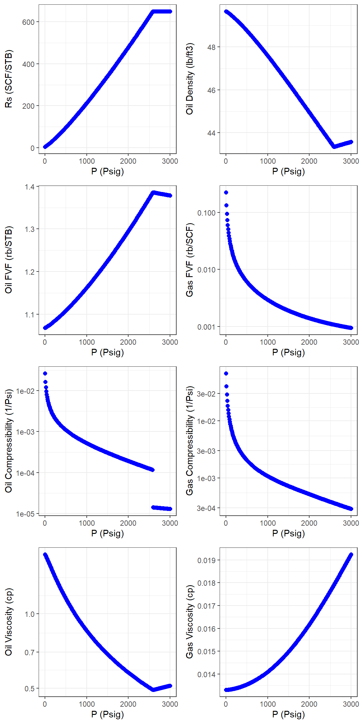
Example 1:
library(Rpvt)
library(ggplot2)
library(magrittr)
library(ggpubr)

pvt_oil_1 <- pvt_oil(input_unit = "Field", output_unit = "Field",
                                   fluid = "black_oil", pvt_model = "Standing",
                                   visc_model = "Beggs_Robinson", t = 200, p = 3000,
                                   oil_api = 35, gas_spgr = 0.8,
                                   nhc_composition = c(0.05,0.02,0.04),
                                   rsi = 650, pb = NULL, warning = "yes")
#> Warning in pvt_oil(input_unit = "Field", output_unit = "Field", fluid =
#> "black_oil", : H2S composition is greater than gas viscosity correlation upper
#> limit: 0.017 mol fraction

attributes(pvt_oil_1)
#> $dim
#> [1] 301  13
#>
#> $dimnames
#> $dimnames[[1]]
#> NULL
#>
#> $dimnames[[2]]
#>  [1] "T_(F)"                "P_(Psig)"             "Rso_(scf/stb)"
#>  [4] "Bo_(rb/stb)"          "Oil_Density_(lb/ft3)" "Co_(1/Psia)"
#>  [7] "Oil_Viscosity_(cp)"   "Z-Factor"             "Bg_(rb/scf)"
#> [10] "Gas_Density_(lb/ft3)" "Cg_(1/Psia)"          "Gas_Viscosity_(cp)"
#> [13] "m(p)_(Psia^2/cp)"
#>
#>
#> $`gas pseudocritical temperature (F)`
#> [1] -61.59983
#>
#> $`gas pseudocritical pressure (Psia)`
#> [1] 647.0921

pvt_oil_1 <- as.data.frame(pvt_oil_1)

tail(pvt_oil_1, 10)
#>     T_(F) P_(Psig) Rso_(scf/stb) Bo_(rb/stb) Oil_Density_(lb/ft3)  Co_(1/Psia)
#> 292   200     2910           650    1.380185             43.52833 1.319029e-05
#> 293   200     2920           650    1.380014             43.53371 1.316513e-05
#> 294   200     2930           650    1.379844             43.53907 1.314019e-05
#> 295   200     2940           650    1.379675             43.54441 1.311547e-05
#> 296   200     2950           650    1.379506             43.54974 1.309097e-05
#> 297   200     2960           650    1.379338             43.55504 1.306667e-05
#> 298   200     2970           650    1.379171             43.56034 1.304258e-05
#> 299   200     2980           650    1.379004             43.56561 1.301870e-05
#> 300   200     2990           650    1.378837             43.57087 1.299502e-05
#> 301   200     3000           650    1.378671             43.57611 1.297154e-05
#>     Oil_Viscosity_(cp)  Z-Factor  Bg_(rb/scf) Gas_Density_(lb/ft3)  Cg_(1/Psia)
#> 292          0.5075536 0.8571989 0.0009737542             11.16752 0.0003017984
#> 293          0.5080544 0.8575451 0.0009708281             11.20118 0.0003001107
#> 294          0.5085569 0.8578959 0.0009679270             11.23475 0.0002984348
#> 295          0.5090612 0.8582513 0.0009650507             11.26824 0.0002967708
#> 296          0.5095672 0.8586112 0.0009621989             11.30164 0.0002951185
#> 297          0.5100750 0.8589757 0.0009593714             11.33495 0.0002934779
#> 298          0.5105844 0.8593446 0.0009565678             11.36817 0.0002918488
#> 299          0.5110956 0.8597181 0.0009537878             11.40130 0.0002902311
#> 300          0.5116085 0.8600959 0.0009510313             11.43435 0.0002886249
#> 301          0.5121231 0.8604782 0.0009482979             11.46731 0.0002870300
#>     Gas_Viscosity_(cp) m(p)_(Psia^2/cp)
#> 292         0.01894741        613123202
#> 293         0.01898046        616726950
#> 294         0.01901354        620335238
#> 295         0.01904666        623948017
#> 296         0.01907980        627565235
#> 297         0.01911298        631186844
#> 298         0.01914620        634812793
#> 299         0.01917944        638443035
#> 300         0.01921272        642077519
#> 301         0.01924602        645716199

Rs_plot <- pvt_oil_1 %>% ggplot(aes(x = `P_(Psig)`, y = `Rso_(scf/stb)`)) +
  geom_point(color = "blue", size = 2) +
  xlab(label = "P (Psig)") +
  ylab(label = "Rs (SCF/STB)") +
  theme_bw()
Bo_plot <- pvt_oil_1 %>% ggplot(aes(x = `P_(Psig)`, y = `Bo_(rb/stb)`)) +
  geom_point(color = "blue", size = 2) +
  xlab(label = "P (Psig)") +
  ylab(label = "Oil FVF (rb/STB)") +
  theme_bw()
RHOo_plot <- pvt_oil_1 %>% ggplot(aes(x = `P_(Psig)`, y = `Oil_Density_(lb/ft3)`)) +
  geom_point(color = "blue", size = 2) +
  xlab(label = "P (Psig)") +
  ylab(label = "Oil Density (lb/ft3)") +
  theme_bw()
Co_plot <- pvt_oil_1 %>% ggplot(aes(x = `P_(Psig)`, y = `Co_(1/Psia)`)) +
  geom_point(color = "blue", size = 2) +
  scale_y_log10() +
  xlab(label = "P (Psig)") +
  ylab(label = "Oil Compressibility (1/Psi)") +
  theme_bw()
MUo_plot <- pvt_oil_1 %>% ggplot(aes(x = `P_(Psig)`, y = `Oil_Viscosity_(cp)`)) +
  geom_point(color = "blue", size = 2) +
  scale_y_log10() +
  xlab(label = "P (Psig)") +
  ylab(label = "Oil Viscosity (cp)") +
  theme_bw()
Bg_plot <- pvt_oil_1 %>% ggplot(aes(x = `P_(Psig)`, y = `Bg_(rb/scf)`)) +
  geom_point(color = "blue", size = 2) +
  scale_y_log10() +
  xlab(label = "P (Psig)") +
  ylab(label = "Gas FVF (rb/SCF)") +
  theme_bw()
Cg_plot <- pvt_oil_1 %>% ggplot(aes(x = `P_(Psig)`, y = `Cg_(1/Psia)`)) +
  geom_point(color = "blue", size = 2) +
  scale_y_log10() +
  xlab(label = "P (Psig)") +
  ylab(label = "Gas Compressibility (1/Psi)") +
  theme_bw()
MUg_plot <- pvt_oil_1 %>% ggplot(aes(x = `P_(Psig)`, y = `Gas_Viscosity_(cp)`)) +
  geom_point(color = "blue", size = 2) +
  xlab(label = "P (Psig)") +
  ylab(label = "Gas Viscosity (cp)") +
  theme_bw()
oil_pvt_plots <- ggarrange(Rs_plot, RHOo_plot, Bo_plot, Bg_plot, Co_plot, Cg_plot, MUo_plot, MUg_plot,
                      ncol = 2, nrow = 4, align = "v")

oil_pvt_plots
Example 2:
pvt_oil_2 <- pvt_oil(input_unit = "SI", output_unit = "SI", fluid = "black_oil",
                     pvt_model = "Vasquez_Beggs", visc_model = "Al_Marhoun",
                     t = 100, p = 20000, oil_api = 40, gas_spgr = 0.75,
                     nhc_composition = c(0.05,0.02,0.04),
                     rsi = NULL, pb = 13000, warning = "yes")
#> Warning in pvt_oil(input_unit = "SI", output_unit = "SI", fluid = "black_oil", :
#> H2S composition is greater than gas viscosity correlation upper limit: 0.017 mol
#> fraction

head(as.data.frame(pvt_oil_2), 10)
#>    T_(C)  P_(kPag) Rso_(rm3/sm3) Bo_(rm3/sm3) Oil_Density_(kg/m3)  Co_(1/kPaa)
#> 1    100   0.00000     0.2401985     1.089818            756.5732 0.0033255930
#> 2    100  68.94757     0.4447876     1.090367            756.3642 0.0021745619
#> 3    100 137.89515     0.6659115     1.090961            756.1386 0.0016446979
#> 4    100 206.84272     0.8994433     1.091588            755.9005 0.0013347696
#> 5    100 275.79029     1.1430314     1.092242            755.6525 0.0011293957
#> 6    100 344.73786     1.3951355     1.092919            755.3962 0.0009823799
#> 7    100 413.68544     1.6546602     1.093616            755.1326 0.0008714483
#> 8    100 482.63301     1.9207823     1.094330            754.8627 0.0007844784
#> 9    100 551.58058     2.1928581     1.095060            754.5871 0.0007142814
#> 10   100 620.52816     2.4703694     1.095805            754.3064 0.0006563117
#>    Oil_Viscosity_(mPa.s)  Z-Factor Bg_(rm3/sm3) Gas_Density_(kg/m3) Cg_(1/kPaa)
#> 1              0.7274220 0.9986855    1.2906979           0.7103805 0.009882170
#> 2              0.7241780 0.9977932    0.7673772           1.1948317 0.005885882
#> 3              0.7206860 0.9969027    0.5457181           1.6801470 0.004193186
#> 4              0.7170347 0.9960140    0.4232449           2.1663262 0.003257910
#> 5              0.7132757 0.9951271    0.3455557           2.6533689 0.002664619
#> 6              0.7094434 0.9942421    0.2918836           3.1412746 0.002254731
#> 7              0.7055623 0.9933590    0.2525829           3.6300428 0.001954588
#> 8              0.7016509 0.9924778    0.2225630           4.1196731 0.001725315
#> 9              0.6977233 0.9915984    0.1988837           4.6101647 0.001544462
#> 10             0.6937909 0.9907210    0.1797282           5.1015171 0.001398153
#>    Gas_Viscosity_(mPa.s) m(p)_(MPaa^2/mPa.s)
#> 1             0.01370328            0.000000
#> 2             0.01370404            1.369056
#> 3             0.01370503            3.434840
#> 4             0.01370622            6.198464
#> 5             0.01370760            9.661007
#> 6             0.01370915           13.823523
#> 7             0.01371087           18.687043
#> 8             0.01371275           24.252573
#> 9             0.01371478           30.521094
#> 10            0.01371695           37.493567
Example 3:
pvt_oil_3 <- pvt_oil(input_unit = "Field", output_unit = "SI", fluid = "black_oil",
                     pvt_model = "Farshad_Petrosky", visc_model = "Al_Marhoun",
                     t = 260, p = 4000, oil_api = 38, gas_spgr = 0.68,
                     nhc_composition = c(0.03,0.07,0.08),
                     rsi = NULL, pb = 2500, warning = "yes")
#> Warning in pvt_oil(input_unit = "Field", output_unit = "SI", fluid =
#> "black_oil", : H2S composition is greater than gas viscosity correlation upper
#> limit: 0.017 mol fraction

head(as.data.frame(pvt_oil_3), 10)
#>       T_(C)  P_(kPag) Rso_(rm3/sm3) Bo_(rm3/sm3) Oil_Density_(kg/m3)
#> 1  126.6667   0.00000      12.46911     1.094699            771.3572
#> 2  126.6667  68.94757      12.62313     1.095295            771.0545
#> 3  126.6667 137.89515      12.77794     1.095892            770.7519
#> 4  126.6667 206.84272      12.93355     1.096491            770.4491
#> 5  126.6667 275.79029      13.08996     1.097091            770.1464
#> 6  126.6667 344.73786      13.24716     1.097692            769.8436
#> 7  126.6667 413.68544      13.40515     1.098295            769.5407
#> 8  126.6667 482.63301      13.56393     1.098899            769.2379
#> 9  126.6667 551.58058      13.72350     1.099505            768.9350
#> 10 126.6667 620.52816      13.88386     1.100112            768.6320
#>     Co_(1/kPaa) Oil_Viscosity_(mPa.s)  Z-Factor Bg_(rm3/sm3)
#> 1  0.0028083871             0.4838329 0.9992613    1.3837332
#> 2  0.0016749541             0.4832363 0.9987608    0.8230142
#> 3  0.0011948412             0.4826397 0.9982621    0.5855144
#> 4  0.0009295394             0.4820430 0.9977651    0.4542889
#> 5  0.0007612280             0.4814463 0.9972700    0.3710476
#> 6  0.0006449318             0.4808496 0.9967766    0.3135399
#> 7  0.0005597603             0.4802529 0.9962850    0.2714305
#> 8  0.0004946890             0.4796564 0.9957953    0.2392652
#> 9  0.0004433500             0.4790600 0.9953074    0.2138937
#> 10 0.0004018085             0.4784638 0.9948213    0.1933693
#>    Gas_Density_(kg/m3) Cg_(1/kPaa) Gas_Viscosity_(mPa.s) m(p)_(MPaa^2/mPa.s)
#> 1            0.6007737 0.009876476            0.01545179            0.000000
#> 2            1.0100805 0.005880180            0.01545242            1.213147
#> 3            1.4197951 0.004187477            0.01545324            3.043021
#> 4            1.8299161 0.003252193            0.01545423            5.490149
#> 5            2.2404418 0.002658895            0.01545537            8.555038
#> 6            2.6513706 0.002249000            0.01545665           12.238176
#> 7            3.0627008 0.001948850            0.01545807           16.540033
#> 8            3.4744308 0.001719571            0.01545962           21.461063
#> 9            3.8865588 0.001538711            0.01546129           27.001701
#> 10           4.2990832 0.001392396            0.01546308           33.162369
Water PVT Examples
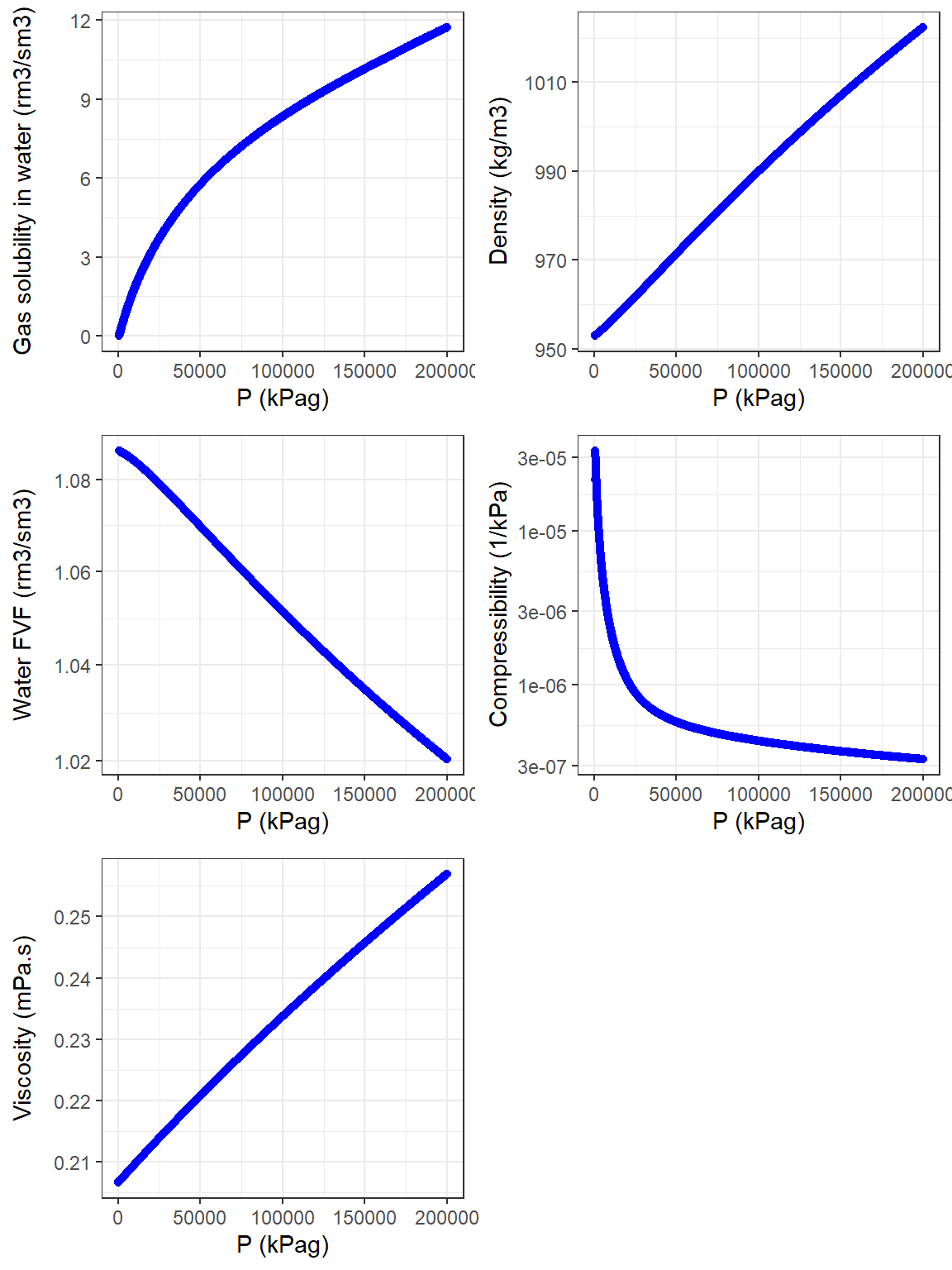
Example 1:
library(Rpvt)
library(ggplot2)
library(magrittr)
library(ggpubr)

pvt_water_1 <- as.data.frame(pvt_water(input_unit = "SI", output_unit = "SI",
fluid = "water", pvt_model = "Spivey", visc_model = "Spivey", t = 150, p = 200000,
salinity = 5, gas_saturated = "yes", warning = "yes"))
#> Warning in pvt_water(input_unit = "SI", output_unit = "SI", fluid = "water", :
#> The pressure lower limit in 'Spivey' correlation is 115 psig (790 kPag)
#> Warning in pvt_water(input_unit = "SI", output_unit = "SI", fluid = "water", :
#> pressure is greater than PVT correlation upper limit: 29000 psig

head(pvt_water_1,10)
#>    T_(C)  P_(kPag) Rsw_(rm3/sm3) Bw_(rm3/sm3) Density_(kg/m3)  Cw_(1/kPaa)
#> 1    150   0.00000           NaN          NaN             NaN          NaN
#> 2    150  68.94757           NaN          NaN             NaN          NaN
#> 3    150 137.89515           NaN          NaN             NaN          NaN
#> 4    150 206.84272           NaN          NaN             NaN          NaN
#> 5    150 275.79029           NaN          NaN             NaN          NaN
#> 6    150 344.73786           NaN          NaN             NaN          NaN
#> 7    150 413.68544   0.001877106     1.086347        952.9482 2.160339e-05
#> 8    150 482.63301   0.009433052     1.086319        952.9771 3.105915e-05
#> 9    150 551.58058   0.019506617     1.086296        953.0035 3.324147e-05
#> 10   150 620.52816   0.031017232     1.086276        953.0285 3.317271e-05
#>    Viscosity_(mPa.s)
#> 1          0.2066466
#> 2          0.2066671
#> 3          0.2066877
#> 4          0.2067082
#> 5          0.2067288
#> 6          0.2067493
#> 7          0.2067698
#> 8          0.2067904
#> 9          0.2068109
#> 10         0.2068314

colnames(pvt_water_1) <- c("T(C)", "P(kPag)", "Rsw(rm3/sm3)", "Bw(rm3/sm3)",
                         "Density(kg/m3)", "Cw(1/kPa)", "MUw(mPa.s)")
Solubility_plot <- pvt_water_1 %>% ggplot(aes(x = `P(kPag)`, y = `Rsw(rm3/sm3)`)) +
  geom_point(color = "blue") +
  xlab(label = "P (kPag)") +
  ylab(label = "Gas solubility in water (rm3/sm3)") +
  theme_bw()
Density_plot <- pvt_water_1 %>% ggplot(aes(x = `P(kPag)`, y = `Density(kg/m3)`)) +
  geom_point(color = "blue") +
  xlab(label = "P (kPag)") +
  ylab(label = "Density (kg/m3)") +
  theme_bw()
Bw_plot <- pvt_water_1 %>% ggplot(aes(x = `P(kPag)`, y = `Bw(rm3/sm3)`)) +
  geom_point(color = "blue") +
  scale_y_log10() +
  xlab(label = "P (kPag)") +
  ylab(label = "Water FVF (rm3/sm3)") +
  theme_bw()
Cw_plot <- pvt_water_1 %>% ggplot(aes(x = `P(kPag)`, y = `Cw(1/kPa)`)) +
  geom_point(color = "blue") +
  scale_y_log10() +
  xlab(label = "P (kPag)") +
  ylab(label = "Compressibility (1/kPa)") +
  theme_bw()
MUw_plot <- pvt_water_1 %>% ggplot(aes(x = `P(kPag)`, y = `MUw(mPa.s)`)) +
  geom_point(color = "blue") +
  xlab(label = "P (kPag)") +
  ylab(label = "Viscosity (mPa.s)") +
  theme_bw()
water_pvt_plots <- ggarrange(Solubility_plot, Density_plot, Bw_plot, Cw_plot, MUw_plot,
                      ncol = 2, nrow = 3, align = "v")
#> Warning: Removed 6 rows containing missing values (geom_point).
#> Warning: Removed 6 rows containing missing values (geom_point).

#> Warning: Removed 6 rows containing missing values (geom_point).

#> Warning: Removed 6 rows containing missing values (geom_point).

water_pvt_plots
Example 2:
pvt_water_2 <- as.data.frame(pvt_water(input_unit = "Field", output_unit = "SI",
fluid = "water", pvt_model = "McCain", visc_model = "McCain", t = 200, p = 4000,
salinity = 15, gas_saturated = "yes", warning = "yes"))

head(pvt_water_2, 10)
#>       T_(C)  P_(kPag) Rsw_(rm3/sm3) Bw_(rm3/sm3) Density_(kg/m3)  Cw_(1/kPaa)
#> 1  93.33333   0.00000     0.1807648     1.038692        1068.840 8.485921e-05
#> 2  93.33333  68.94757     0.1855351     1.038684        1068.848 5.056644e-05
#> 3  93.33333 137.89515     0.1903012     1.038676        1068.856 3.604131e-05
#> 4  93.33333 206.84272     0.1950633     1.038668        1068.864 2.801577e-05
#> 5  93.33333 275.79029     0.1998212     1.038660        1068.872 2.292487e-05
#> 6  93.33333 344.73786     0.2045751     1.038652        1068.881 1.940781e-05
#> 7  93.33333 413.68544     0.2093249     1.038644        1068.889 1.683249e-05
#> 8  93.33333 482.63301     0.2140705     1.038635        1068.898 1.486533e-05
#> 9  93.33333 551.58058     0.2188121     1.038627        1068.906 1.331367e-05
#> 10 93.33333 620.52816     0.2235496     1.038619        1068.915 1.205845e-05
#>    Viscosity_(mPa.s)
#> 1          0.4528099
#> 2          0.4529929
#> 3          0.4531762
#> 4          0.4533598
#> 5          0.4535436
#> 6          0.4537278
#> 7          0.4539122
#> 8          0.4540969
#> 9          0.4542819
#> 10         0.4544672
Example 3:
pvt_water_3 <- pvt_water(input_unit = "Field", output_unit = "Field",
fluid = "water", pvt_model = "Meehan", visc_model = "Meehan",
t = 300, p = 3000,  salinity = 10, gas_saturated = "no", warning = "yes")
#> Warning in pvt_water(input_unit = "Field", output_unit = "Field", fluid =
#> "water", : temperature is greater than PVT correlation upper limit: 250 F

tail(as.data.frame(pvt_water_3), 10)
#>     T_(F) P_(Psig) Rsw_(scf/stb) Bw_(rb/stb) Density_(lb/ft3)  Cw_(1/Psia)
#> 292   300     2910             0    1.072288         62.40311 3.152895e-06
#> 293   300     2920             0    1.072257         62.40493 3.152346e-06
#> 294   300     2930             0    1.072225         62.40676 3.151797e-06
#> 295   300     2940             0    1.072194         62.40858 3.151249e-06
#> 296   300     2950             0    1.072163         62.41040 3.150700e-06
#> 297   300     2960             0    1.072131         62.41223 3.150151e-06
#> 298   300     2970             0    1.072100         62.41405 3.149602e-06
#> 299   300     2980             0    1.072069         62.41587 3.149054e-06
#> 300   300     2990             0    1.072038         62.41768 3.148505e-06
#> 301   300     3000             0    1.072006         62.41950 3.147956e-06
#>     Viscosity_(cp)
#> 292      0.2781652
#> 293      0.2781799
#> 294      0.2781947
#> 295      0.2782095
#> 296      0.2782244
#> 297      0.2782393
#> 298      0.2782542
#> 299      0.2782693
#> 300      0.2782843
#> 301      0.2782994
References
Al-Marhoun, M. A. (1988). PVT Correlations for Middle East Crude Oils. Journal of Petroleum Technology, 40(05), 650–666. https://doi.org/10.2118/13718-PA
Al-Marhoun, M. A. (2004). Evaluation of empirically derived PVT properties for Middle East crude oils. Journal of Petroleum Science and Engineering, 42(2), 209–221.
Beggs, H. D., & Robinson, J. R. (1975). Estimating the Viscosity of Crude Oil Systems. Journal of Petroleum Technology, 27(09), 1140–1141. https://doi.org/10.2118/5434-PA
Glaso, O. (1980). Generalized Pressure-Volume-Temperature Correlations. Journal of Petroleum Technology, 32(05), 785–795. https://doi.org/10.2118/8016-PA
McCain, Jr., W. D., Spivey, J. P., & Lenn, C. P. (2011). Petroleum Reservoir Fluid Property Correlations (p. 219). PennWell Corporation.
McCain Jr., W. D. (1991). Reservoir-Fluid Property Correlations-State of the Art (includes associated papers 23583 and 23594 ). SPE Reservoir Engineering, 6(02), 266–272. https://doi.org/10.2118/18571-PA
Meehan, D. N. (1980a). A correlation for water compressibility. Petroleum Engineer, 56, 125–126.
Meehan, D. N. (1980b). Estimating water viscosity at reservoir conditions. Petroleum Engineer, 35, 117–118.
Petrosky Jr., G. E., & Farshad, F. (1998). Pressure-Volume-Temperature Correlations for Gulf of Mexico Crude Oils. SPE Reservoir Evaluation & Engineering, 1(05), 416–420. https://doi.org/10.2118/51395-PA
Spivey, J. P., McCain, W. D., & North, R. (2004). Estimating density, formation volume factor, compressibility, methane solubility, and viscosity for oilfield brines at temperatures from 0 to 275° C, pressures to 200 MPa, and salinities to 5.7 mole/kg. Journal of Canadian Petroleum Technology, 43(7), 52–61. https://doi.org/10.2118/04-07-05
Spivey, J. P., Valko, P. P., & McCain, W. D. (2007). Applications of the Coefficient of Isothermal Compressibility to Various Reservoir Situations With New Correlations for Each Situation. SPE Reservoir Evaluation & Engineering, 10(01), 43–49. https://doi.org/10.2118/96415-PA
Standing, M. B. (1947). A Pressure-Volume-Temperature Correlation For Mixtures Of California Oils And Gases. New York, New York: American Petroleum Institute.
Sutton, R. P. (2007). Fundamental PVT Calculations for Associated and Gas/Condensate Natural-Gas Systems. SPE Reservoir Evaluation & Engineering, 10(03), 270–284. https://doi.org/10.2118/97099-PA
Vasquez, M., & Beggs, H. D. (1980). Correlations for Fluid Physical Property Prediction. Journal of Petroleum Technology, 32(06), 968–970. https://doi.org/10.2118/6719-PA