Material Balance - Dry and Wet Gas Reservoirs
DryWetGas.Rmd
Examples
Example 1: Dry Gas Reservoir (Ikoku, Chi, 1984)
Part I: History Match
library(Rmbal)
library(Rrelperm)
library(pracma)
library(minpack.lm)
library(ggplot2)
library(dplyr)
#>
#> Attaching package: 'dplyr'
#> The following objects are masked from 'package:stats':
#>
#>     filter, lag
#> The following objects are masked from 'package:base':
#>
#>     intersect, setdiff, setequal, union
library(magrittr)
#>
#> Attaching package: 'magrittr'
#> The following objects are masked from 'package:pracma':
#>
#>     and, mod, or

p_pvt <- c(1798, 1680, 1540, 1428, 1335)                 # psia

Bg <- c(0.00152, 0.00163, 0.00179, 0.00196, 0.00210)     # RB/SCF

Bo <- rep(0, length(p_pvt))    # RB/STB

Rv <- rep(0, length(p_pvt))    # STB/SCF

Rs <- rep(1e8, length(p_pvt))  # SCF/STB

Bw <- rep(1, length(p_pvt))    # RB/STB

muo <- rep(0.5, length(p_pvt))              # cp

muw <- rep(0.25, length(p_pvt))             # cp

mug <- rep(0.015, length(p_pvt))            # cp

pvt_table <- data.frame(p = p_pvt, Bo = Bo, Rs = Rs, Rv = Rv, Bg = Bg,
                             Bw = Bw, muo = muo, mug = mug, muw = muw)

p <- c(1798, 1680, 1540, 1428, 1335)

Np <- rep(0, length.out = length(p))

Gp <- c(0, 0.96, 2.12, 3.21, 3.92) * 1e9    # SCF

Wp <- rep(0, length.out = length(p))

We <- rep(0, length.out = length(p))

Wi <- rep(0, length.out = length(p))

wf <- rep(1, length.out = length(p))

mbal_optim_gas_lst <- mbal_optim_param_gas(input_unit = "Field", output_unit = "Field",
                                          unknown_param = "G", aquifer_model = NULL,
                                          G = NULL, phi = 0.13, swi = 0.52,
                                          Np = Np, Gp = Gp, Wp = Wp, Wi = Wi,
                                          We = We, pd = 0, p = p, pvt = pvt_table,
                                          M = 0, cf = 3e-6, wf = wf, sgrw = 0.0)

time_lst <- mbal_time(c(0, 0.5, 1.0, 1.5, 2.0), "year")

# a number of plots will be automatically generated for quality check

optim_results <- mbal_optim_gas(mbal_optim_gas_lst, time_lst)
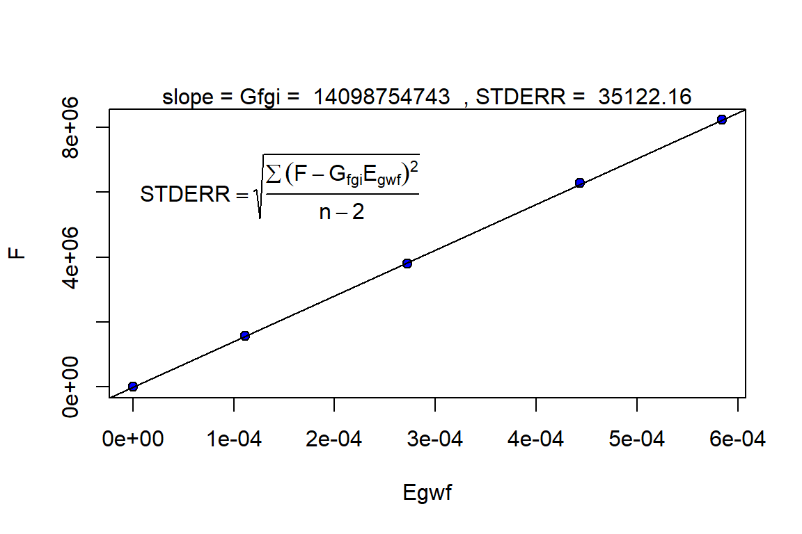
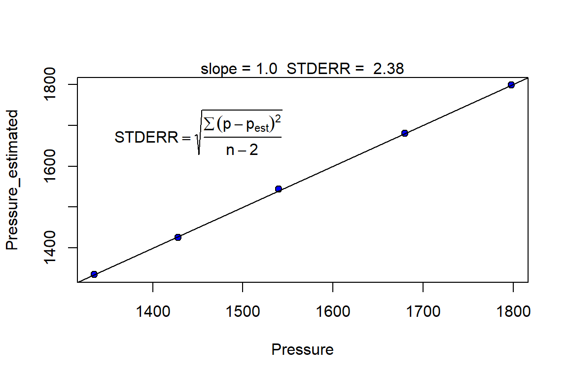
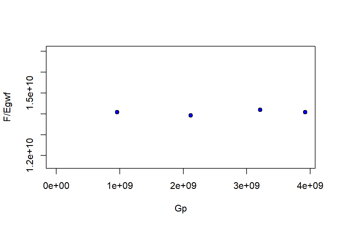
glimpse(optim_results)
#> List of 17
#>  $ input_unit : chr "Field"
#>  $ output_unit: chr "Field"
#>  $ G          : num 1.41e+10
#>  $ phi        : num 0.13
#>  $ swi        : num 0.52
#>  $ pd         : num 0
#>  $ p          : num [1:5] 1798 1680 1540 1428 1335
#>  $ cf         : num [1:5] 3e-06 3e-06 3e-06 3e-06 3e-06
#>  $ M          : num 0
#>  $ pvt        :'data.frame': 5 obs. of  9 variables:
#>   ..$ p  : num [1:5] 1798 1680 1540 1428 1335
#>   ..$ Bo : num [1:5] 0 0 0 0 0
#>   ..$ Rs : num [1:5] 1e+08 1e+08 1e+08 1e+08 1e+08
#>   ..$ Rv : num [1:5] 0 0 0 0 0
#>   ..$ Bg : num [1:5] 0.00152 0.00163 0.00179 0.00196 0.0021
#>   ..$ Bw : num [1:5] 1 1 1 1 1
#>   ..$ muo: num [1:5] 0.5 0.5 0.5 0.5 0.5
#>   ..$ mug: num [1:5] 0.015 0.015 0.015 0.015 0.015
#>   ..$ muw: num [1:5] 0.25 0.25 0.25 0.25 0.25
#>  $ prod       :'data.frame': 5 obs. of  3 variables:
#>   ..$ Np: num [1:5] 0 0 0 0 0
#>   ..$ Gp: num [1:5] 0.00 9.60e+08 2.12e+09 3.21e+09 3.92e+09
#>   ..$ Wp: num [1:5] 0 0 0 0 0
#>  $ inj        :'data.frame': 5 obs. of  1 variable:
#>   ..$ Wi: num [1:5] 0 0 0 0 0
#>  $ We         : num [1:5] 0 0 0 0 0
#>  $ aquifer    :List of 3
#>   ..$ input_unit : chr "Field"
#>   ..$ output_unit: chr "Field"
#>   ..$ We         : num [1:5] 0 0 0 0 0
#>   ..- attr(*, "class")= chr [1:2] "NoA" "aquifer"
#>  $ wf         : num [1:5] 1 1 1 1 1
#>  $ sgrw       : num 0
#>  $ p_est      : num [1:5] 1798 1680 1543 1426 1335
#>  - attr(*, "class")= chr [1:2] "volumetric_gas" "mbal_gas"
Part II: Reservoir Performance
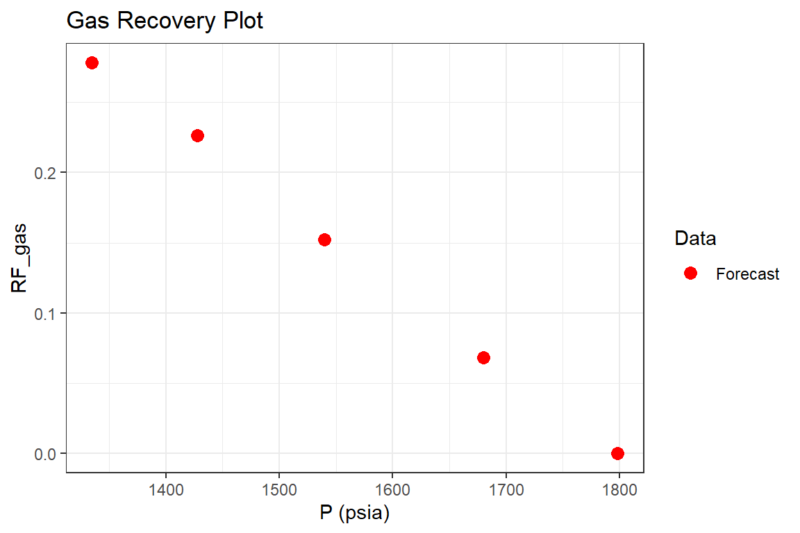
mbal_results <- mbal_perform_gas(optim_results, time_lst)

mbal_results
#>   P (psia) Eo (bbl/STB) Eg (bbl/SCF) Ew (bbl/STB) Ef (bbl/bbl) Egwf (bbl/SCF)
#> 1     1798            0      0.00000            0     0.000000   0.0000000000
#> 2     1680            0      0.00011            0     0.000354   0.0001111210
#> 3     1540            0      0.00027            0     0.000774   0.0002724510
#> 4     1428            0      0.00044            0     0.001110   0.0004435150
#> 5     1335            0      0.00058            0     0.001389   0.0005843985
#>   Et (bbl) F (bbl) We       Igd Inwd        Ifwd Iawd Itot     RF_oil
#> 1        0       0  0        NA   NA          NA   NA   NA 0.00000000
#> 2  1566668 1564800  0 0.9899119    0 0.010088102    0    1 0.06817239
#> 3  3841220 3794800  0 0.9910039    0 0.008996113    0    1 0.15220726
#> 4  6253009 6291600  0 0.9920747    0 0.007925324    0    1 0.22628316
#> 5  8239291 8232000  0 0.9924735    0 0.007526542    0    1 0.27828500
#>       RF_gas SOg  SGg  SWg SOT  SGT  SWT qo (STB/day) qg (SCF/day) qw (STB/day)
#> 1 0.00000000   0 0.48 0.52   0 0.48 0.52            0            0            0
#> 2 0.06817239   0 0.48 0.52   0 0.48 0.52            0      5260274            0
#> 3 0.15220726   0 0.48 0.52   0 0.48 0.52            0      6356164            0
#> 4 0.22628316   0 0.48 0.52   0 0.48 0.52            0      5972603            0
#> 5 0.27828500   0 0.48 0.52   0 0.48 0.52            0      3890411            0
#>   fo fw GOR (SCF/STB) kro/krg
#> 1  0  0           Inf       0
#> 2  0  0           Inf       0
#> 3  0  0           Inf       0
#> 4  0  0           Inf       0
#> 5  0  0           Inf       0

p1 <- mbal_results %>% ggplot(aes(`P (psia)`, `RF_gas`, color = "Forecast")) +
  geom_point(size = 3) +
  scale_color_manual(name="Data", values=c("Forecast" = "red")) +
  ggtitle("Gas Recovery Plot") +
  theme_bw()

p1
p2 <- mbal_results  %>%
  tidyr::pivot_longer(cols = c("Igd", "Ifwd"), names_to = "Drive Mechanism",
                      values_to = "Fraction", values_drop_na = TRUE) %>%
  ggplot(aes(`P (psia)`, Fraction, fill = `Drive Mechanism`)) +
  geom_area() +
  ggtitle("Energy Plot") +
  theme_bw()

p2

Part III: Reservoir Forecast
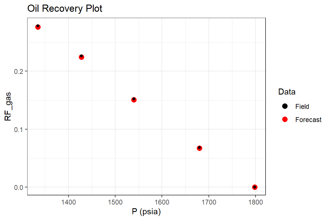
# gas saturation above the bubble point is zero, however the mbal_forecast_param_oil()
# requires a table of relative permeabilities as an input for the gas-oil system.
# Therefore, an arbitrary table is generated using the 'Rrelperm' package.
# The generated table does not impact the predictions above the bubble point.


rel_perm <- as.data.frame(Rrelperm::kr2p_gl(SWCON = 0.52, SOIRG = 0.15, SORG = 0.15,
                                            SGCON = 0.05, SGCRIT = 0.05, KRGCL = 1,
                                            KROGCG = 1, NG = 1, NOG = 1.0, NP = 101))

colnames(rel_perm) <- c("Sg", "Sl", "Krg", "Krog")

forecast_lst <- mbal_forecast_param_gas(input_unit = "Field", output_unit = "Field",
                                        G = 1.41e10, phi = 0.13, swi = 0.52, pd = 0,
                                        p = p, pvt = pvt_table, M = 0, cf = 3e-6,
                                        wf = wf, rel_perm = rel_perm)

glimpse(forecast_lst)
#> List of 12
#>  $ input_unit : chr "Field"
#>  $ output_unit: chr "Field"
#>  $ G          : num 1.41e+10
#>  $ phi        : num 0.13
#>  $ swi        : num 0.52
#>  $ pd         : num 0
#>  $ p          : num [1:5] 1798 1680 1540 1428 1335
#>  $ cf         : num [1:5] 3e-06 3e-06 3e-06 3e-06 3e-06
#>  $ M          : num 0
#>  $ pvt        :'data.frame': 5 obs. of  9 variables:
#>   ..$ p  : num [1:5] 1798 1680 1540 1428 1335
#>   ..$ Bo : num [1:5] 0 0 0 0 0
#>   ..$ Rs : num [1:5] 1e+08 1e+08 1e+08 1e+08 1e+08
#>   ..$ Rv : num [1:5] 0 0 0 0 0
#>   ..$ Bg : num [1:5] 0.00152 0.00163 0.00179 0.00196 0.0021
#>   ..$ Bw : num [1:5] 1 1 1 1 1
#>   ..$ muo: num [1:5] 0.5 0.5 0.5 0.5 0.5
#>   ..$ mug: num [1:5] 0.015 0.015 0.015 0.015 0.015
#>   ..$ muw: num [1:5] 0.25 0.25 0.25 0.25 0.25
#>  $ wf         : num [1:5] 1 1 1 1 1
#>  $ rel_perm   :'data.frame': 101 obs. of  4 variables:
#>   ..$ Sg  : num [1:101] 0 0.01 0.02 0.03 0.04 0.05 0.06 0.07 0.08 0.09 ...
#>   ..$ Sl  : num [1:101] 1 0.99 0.98 0.97 0.96 0.95 0.94 0.93 0.92 0.91 ...
#>   ..$ Krg : num [1:101] 0 0 0 0 0 ...
#>   ..$ Krog: num [1:101] 1 1 1 1 1 ...
#>  - attr(*, "class")= chr [1:2] "volumetric_forecast_gas" "forecast_gas"

forecast_results <- mbal_forecast_gas(forecast_lst, time_lst)

forecast_results
#>   P (psia) SOg  SGg  SWg SOT  SGT  SWT GOR (SCF/STB)     RF_oil     RF_gas
#> 1     1798   0 0.48 0.52   0 0.48 0.52           Inf 0.00000000 0.00000000
#> 2     1680   0 0.48 0.52   0 0.48 0.52           Inf 0.06748466 0.06748466
#> 3     1540   0 0.48 0.52   0 0.48 0.52           Inf 0.15083799 0.15083799
#> 4     1428   0 0.48 0.52   0 0.48 0.52           Inf 0.22448980 0.22448980
#> 5     1335   0 0.48 0.52   0 0.48 0.52           Inf 0.27619048 0.27619048
#>   Liq_volume       Igd Inwd        Ifwd Iawd Itot
#> 1          0        NA   NA          NA   NA   NA
#> 2          0 0.9899119    0 0.010088102    0    1
#> 3          0 0.9910039    0 0.008996113    0    1
#> 4          0 0.9920747    0 0.007925324    0    1
#> 5          0 0.9924735    0 0.007526542    0    1

p1 <- forecast_results %>% ggplot(aes(`P (psia)`, `RF_gas`, color = "Forecast")) +
  geom_point(size = 3) +
  geom_point(data = mbal_results, aes(`P (psia)`, `RF_gas`, color = "Field"))+
  scale_color_manual(name="Data", values=c("Forecast" = "red", "Field" = "black")) +
  ggtitle("Oil Recovery Plot") +
  theme_bw()

p1
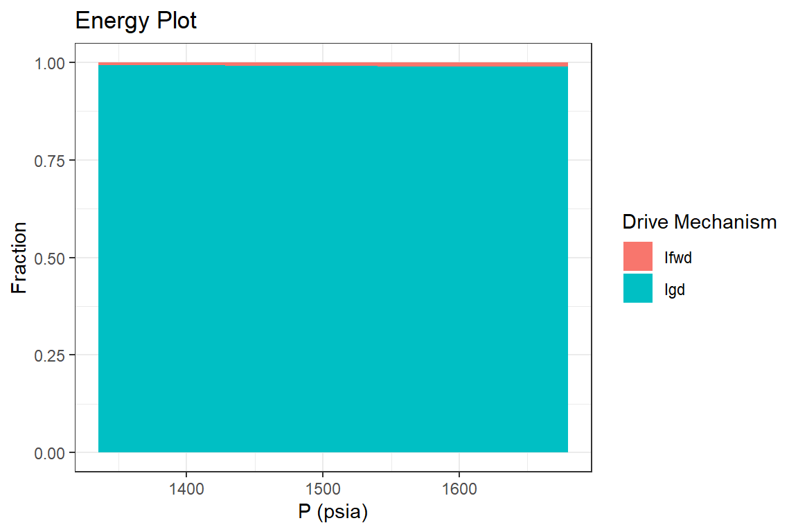
p2 <- forecast_results  %>%
  tidyr::pivot_longer(cols = c("Igd", "Ifwd"), names_to = "Drive Mechanism",
                      values_to = "Fraction", values_drop_na = TRUE) %>%
  ggplot(aes(`P (psia)`, Fraction, fill = `Drive Mechanism`)) +
  geom_area() +
  ggtitle("Energy Plot") +
  theme_bw()

p2
Example 2: Dry Gas Reservoir with Aquifer (Pletcher, 2002)
Part I: History Match
library(Rmbal)
library(Rrelperm)
library(pracma)
library(minpack.lm)
library(ggplot2)
library(dplyr)
library(magrittr)

p_pvt <- c(6411, 5947, 5509, 5093, 4697, 4319, 3957, 3610, 3276, 2953, 2638)

Bg <- c(6279, 6587, 6933, 7327, 7778, 8300, 8910, 9628, 10487, 11532,
        12829) / 10000   # RB/SCF

Bo <- rep(0, length(p_pvt))    # RB/STB

Rv <- rep(0, length(p_pvt))    # STB/SCF

Rs <- rep(1e8, length(p_pvt))  # SCF/STB

Bw <- c(1.0452, 1.0467, 1.0480, 1.0493, 1.0506, 1.0517, 1.0529, 1.0540, 1.0551,
        1.0560, 1.0571)        # RB/STB

muo <- rep(0.5, length(p_pvt))               # cp

muw <- rep(0.25, length(p_pvt))              # cp

mug <- rep(0.025, length(p_pvt))             # cp

pvt_table <- data.frame(p = p_pvt, Bo = Bo, Rs = Rs, Rv = Rv, Bg = Bg,
                             Bw = Bw, muo = muo, mug = mug, muw = muw)

p <- c(6411, 5947, 5509, 5093, 4697, 4319, 3957, 3610, 3276, 2953, 2638)   # psia

Np <- rep(0, length.out = length(p))

Gp <- c(0, 5.475, 10.950, 16.425, 21.900, 27.375, 32.850, 38.325, 43.800, 49.275,
        54.750) * 1e9                                                      # SCF

Wp <- c(0, 378, 1434, 3056, 5284, 8183, 11864, 16425, 22019, 28860, 37256) # STB

Wi <- rep(0, length.out = length(p))

wf <- rep(1, length.out = length(p))

mbal_optim_gas_lst <- mbal_optim_param_gas(input_unit = "Field", output_unit = "Field",
                                          unknown_param = "We", aquifer_model = "pot",
                                          G = 101e9, phi = 0.15, swi = 0.15,
                                          Np = Np, Gp = Gp, Wp = Wp, Wi = Wi,
                                          We = NULL, pd = 0, p = p, pvt = pvt_table,
                                          M = 0, cf = 6e-6, wf = wf, sgrw = 0.0,
                                          phi_a = 0.15, h_a = 200, r_a = 500,
                                          r_R = 210.6, tetha = 360, cw_a = 3e-6,
                                          cf_a = 6e-6, mult_len = 2)

time_lst <- mbal_time(c(1:length(p)), "year")

# a number of plots will be automatically generated for quality check

optim_results <- mbal_optim_gas(mbal_optim_gas_lst, time_lst)
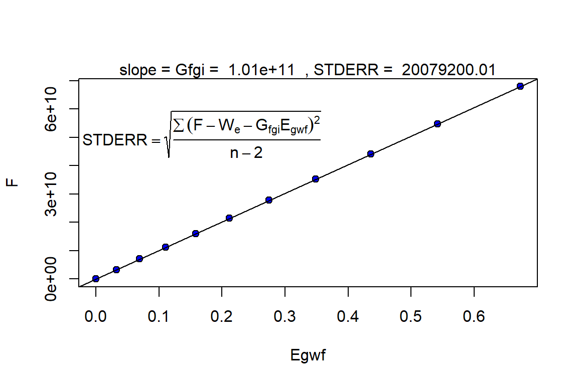
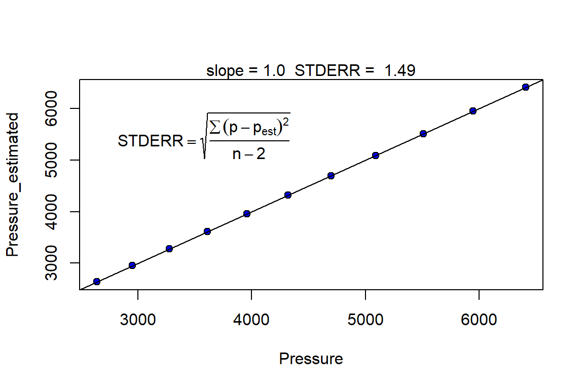
glimpse(optim_results)
#> List of 17
#>  $ input_unit : chr "Field"
#>  $ output_unit: chr "Field"
#>  $ G          : num 1.01e+11
#>  $ phi        : num 0.15
#>  $ swi        : num 0.15
#>  $ pd         : num 0
#>  $ p          : num [1:11] 6411 5947 5509 5093 4697 ...
#>  $ cf         : num [1:11] 6e-06 6e-06 6e-06 6e-06 6e-06 6e-06 6e-06 6e-06 6e-06 6e-06 ...
#>  $ M          : num 0
#>  $ pvt        :'data.frame': 11 obs. of  9 variables:
#>   ..$ p  : num [1:11] 6411 5947 5509 5093 4697 ...
#>   ..$ Bo : num [1:11] 0 0 0 0 0 0 0 0 0 0 ...
#>   ..$ Rs : num [1:11] 1e+08 1e+08 1e+08 1e+08 1e+08 1e+08 1e+08 1e+08 1e+08 1e+08 ...
#>   ..$ Rv : num [1:11] 0 0 0 0 0 0 0 0 0 0 ...
#>   ..$ Bg : num [1:11] 0.628 0.659 0.693 0.733 0.778 ...
#>   ..$ Bw : num [1:11] 1.05 1.05 1.05 1.05 1.05 ...
#>   ..$ muo: num [1:11] 0.5 0.5 0.5 0.5 0.5 0.5 0.5 0.5 0.5 0.5 ...
#>   ..$ mug: num [1:11] 0.025 0.025 0.025 0.025 0.025 0.025 0.025 0.025 0.025 0.025 ...
#>   ..$ muw: num [1:11] 0.25 0.25 0.25 0.25 0.25 0.25 0.25 0.25 0.25 0.25 ...
#>  $ prod       :'data.frame': 11 obs. of  3 variables:
#>   ..$ Np: num [1:11] 0 0 0 0 0 0 0 0 0 0 ...
#>   ..$ Gp: num [1:11] 0.00 5.48e+09 1.10e+10 1.64e+10 2.19e+10 ...
#>   ..$ Wp: num [1:11] 0 378 1434 3056 5284 ...
#>  $ inj        :'data.frame': 11 obs. of  1 variable:
#>   ..$ Wi: num [1:11] 0 0 0 0 0 0 0 0 0 0 ...
#>  $ We         : NULL
#>  $ aquifer    :List of 12
#>   ..$ input_unit : chr "Field"
#>   ..$ output_unit: chr "Field"
#>   ..$ model      : chr "pot"
#>   ..$ phi        : num 0.15
#>   ..$ h_a        : num 200
#>   ..$ r_a        : num 63512
#>   ..$ r_R        : num 211
#>   ..$ tetha      : num 360
#>   ..$ c_water    : num 3e-06
#>   ..$ c_rock     : num 6e-06
#>   ..$ pressure   : num [1:11] 6411 5947 5509 5093 4697 ...
#>   ..$ mult_len   : num 1
#>   ..- attr(*, "class")= chr [1:2] "pot" "aquifer"
#>  $ wf         : num [1:11] 1 1 1 1 1 1 1 1 1 1 ...
#>  $ sgrw       : num 0
#>  $ p_est      : num [1:11] 6411 5949 5509 5092 4695 ...
#>  - attr(*, "class")= chr [1:2] "water_drive_gas" "mbal_gas"
Part II: Reservoir Performance
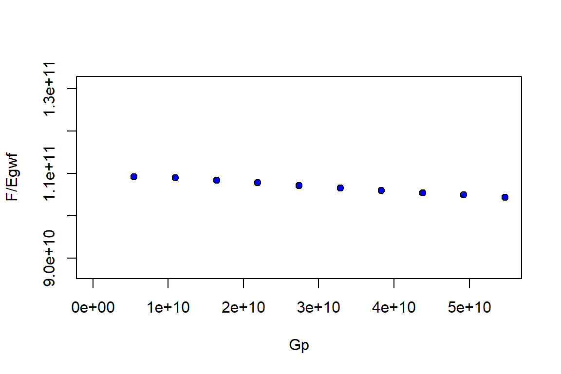
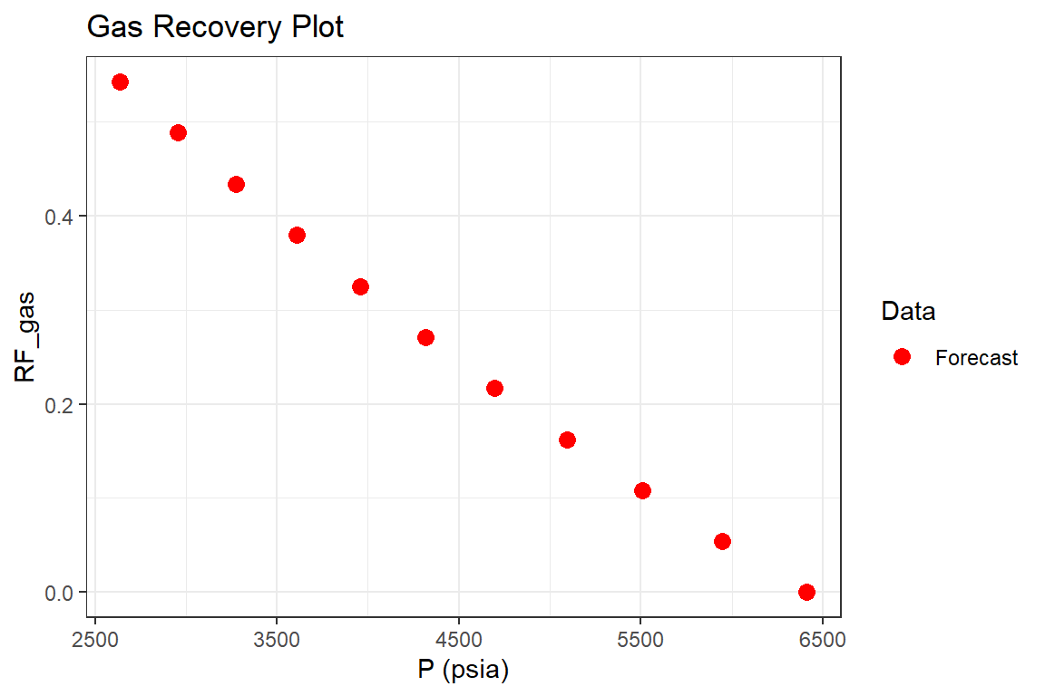
mbal_results <- mbal_perform_gas(optim_results, time_lst)

mbal_results
#>    P (psia) Eo (bbl/STB) Eg (bbl/SCF) Ew (bbl/STB) Ef (bbl/bbl) Egwf (bbl/SCF)
#> 1      6411            0       0.0000       0.0000     0.000000     0.00000000
#> 2      5947            0       0.0308       0.0015     0.002784     0.03301558
#> 3      5509            0       0.0654       0.0028     0.005412     0.06969472
#> 4      5093            0       0.1048       0.0041     0.007908     0.11107634
#> 5      4697            0       0.1499       0.0054     0.010284     0.15806933
#> 6      4319            0       0.2021       0.0065     0.012552     0.21206133
#> 7      3957            0       0.2631       0.0077     0.014724     0.27479301
#> 8      3610            0       0.3349       0.0088     0.016806     0.34824761
#> 9      3276            0       0.4208       0.0099     0.018810     0.43574460
#> 10     2953            0       0.5253       0.0108     0.020748     0.54177162
#> 11     2638            0       0.6550       0.0119     0.022638     0.67298439
#>       Et (bbl)     F (bbl)         We       Igd       Inwd       Ifwd
#> 1            0           0          0        NA         NA         NA
#> 2   3617316708  3606382896  282743700 0.8599745 0.07816393 0.06186171
#> 3   7588808773  7591636503  549644004 0.8704133 0.07242823 0.05715868
#> 4  12021845864 12034600707  803138356 0.8804638 0.06680658 0.05272990
#> 5  17009441970 17033825551 1044445479 0.8900880 0.06140387 0.04850847
#> 6  22692969573 22721258606 1274784097 0.8994900 0.05617529 0.04433506
#> 7  29249454812 29269362492 1495372932 0.9084990 0.05112481 0.04037663
#> 8  36879813117 36899327312 1706821346 0.9171657 0.04628064 0.03655412
#> 9  45920529098 45933083232 1910348062 0.9255294 0.04160118 0.03286992
#> 10 56826075082 56823960476 2107171801 0.9336436 0.03708107 0.02927589
#> 11 70270504750 70238814383 2299120650 0.9414334 0.03271815 0.02584902
#>             Iawd Itot     RF_oil     RF_gas SOg  SGg  SWg SOT       SGT
#> 1             NA   NA 0.00000000 0.00000000   0 0.85 0.15   0 0.8500000
#> 2  -1.093774e-07    1 0.05437227 0.05437227   0 0.85 0.15   0 0.8462103
#> 3  -1.980327e-07    1 0.10837548 0.10837548   0 0.85 0.15   0 0.8426331
#> 4  -2.667361e-07    1 0.16245145 0.16245145   0 0.85 0.15   0 0.8392355
#> 5  -3.263699e-07    1 0.21652136 0.21652136   0 0.85 0.15   0 0.8360012
#> 6  -3.792391e-07    1 0.27070225 0.27070225   0 0.85 0.15   0 0.8329140
#> 7  -4.270714e-07    1 0.32502645 0.32502645   0 0.85 0.15   0 0.8299575
#> 8  -4.694153e-07    1 0.37925495 0.37925495   0 0.85 0.15   0 0.8271234
#> 9  -5.059229e-07    1 0.43354506 0.43354506   0 0.85 0.15   0 0.8243956
#> 10 -5.363059e-07    1 0.48788970 0.48788970   0 0.85 0.15   0 0.8217577
#> 11 -5.604530e-07    1 0.54232409 0.54232409   0 0.85 0.15   0 0.8191851
#>          SWT qo (STB/day) qg (SCF/day) qw (STB/day) fo           fw
#> 1  0.1500000            0      0.0e+00     0.000000  0 0.000000e+00
#> 2  0.1537897            0      1.5e+07     1.035616  0 1.097090e-07
#> 3  0.1573669            0      1.5e+07     2.893151  0 2.915545e-07
#> 4  0.1607645            0      1.5e+07     4.443836  0 4.242678e-07
#> 5  0.1639988            0      1.5e+07     6.104110  0 5.496678e-07
#> 6  0.1670860            0      1.5e+07     7.942466  0 6.709306e-07
#> 7  0.1700425            0      1.5e+07    10.084932  0 7.944943e-07
#> 8  0.1728766            0      1.5e+07    12.495890  0 9.119690e-07
#> 9  0.1756044            0      1.5e+07    15.326027  0 1.027970e-06
#> 10 0.1782423            0      1.5e+07    18.742466  0 1.144180e-06
#> 11 0.1808149            0      1.5e+07    23.002740  0 1.263604e-06
#>    GOR (SCF/STB) kro/krg
#> 1            Inf       0
#> 2            Inf       0
#> 3            Inf       0
#> 4            Inf       0
#> 5            Inf       0
#> 6            Inf       0
#> 7            Inf       0
#> 8            Inf       0
#> 9            Inf       0
#> 10           Inf       0
#> 11           Inf       0

p1 <- mbal_results %>% ggplot(aes(`P (psia)`, `RF_gas`, color = "Forecast")) +
  geom_point(size = 3) +
  scale_color_manual(name="Data", values=c("Forecast" = "red")) +
  ggtitle("Gas Recovery Plot") +
  theme_bw()

p1
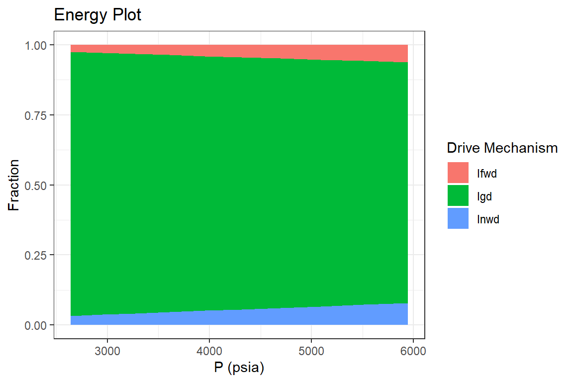
p2 <- mbal_results  %>%
  tidyr::pivot_longer(cols = c("Inwd", "Igd", "Ifwd"), names_to = "Drive Mechanism",
                      values_to = "Fraction", values_drop_na = TRUE) %>%
  ggplot(aes(`P (psia)`, Fraction, fill = `Drive Mechanism`)) +
  geom_area() +
  ggtitle("Energy Plot") +
  theme_bw()

p2
Example 3: Wet Gas Reservoir (Walsh & Lake, 2003)
Part I: Reservoir Forecast
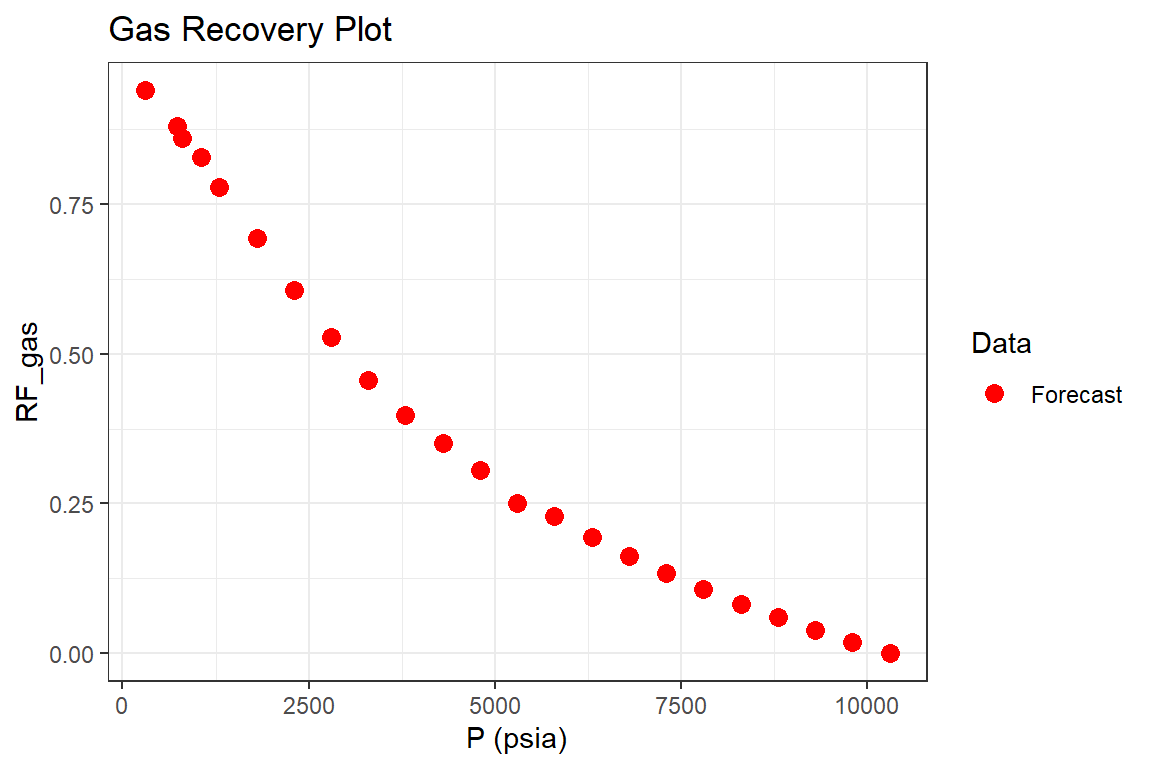
library(Rmbal)
library(Rrelperm)
library(pracma)
library(minpack.lm)
library(ggplot2)
library(dplyr)
library(magrittr)

p_pvt <- c(10300, 9800, 9300, 8800, 8300, 7800, 7300, 6800, 6300, 5800, 5300, 4800,
         4300, 3800, 3300, 2800, 2300, 1800, 1300, 1050, 800, 738, 300) # psia

Bg <- c(0.5, 0.51, 0.52, 0.532, 0.545, 0.560, 0.577, 0.597, 0.621, 0.648, 0.668,
      0.72, 0.77, 0.83, 0.92, 1.06, 1.27, 1.63, 2.26, 2.925, 3.59,
      4.19, 8.39) / 1000                                                # RB/SCF

Bo <- c(18.62, 18.97, 19.36, 19.8, 20.20, 20.85, 21.49, 22.23, 23.11, 24.15, 25.31,
      26.80, 28.66, 30.89, 34.24, 39.45, 47.26, 60.66, 84.11, 108.86, 133.60,
      155.93, 312.24)                                                   # RB/STB

Rv <- rep(26.9, length(p_pvt)) / 1e6                                    # STB/SCF

Rs <- rep(37216, length(p_pvt))                                         # SCF/STB

cw <- 2e-6

Bwi <- 1.0

Bw <- Bwi * exp(cw * (p_pvt[1] - p_pvt))       # RB/STB

muo <- rep(0.5, length(p_pvt))                 # cp

muw <- rep(0.25, length(p_pvt))                # cp

mug <- c(0.047, 0.0455, 0.044, 0.0425, 0.041, 0.00395, 0.0379, 0.0363, 0.0347,
         0.033, 0.0311, 0.0289, 0.02267, 0.0243, 0.0220, 0.0197, 0.0177, 0.0160,
         0.0147, 0.0142, 0.0138, 0.0136, 0.0128)      # cp

pvt_table <- data.frame(p = p_pvt, Bo = Bo, Rs = Rs, Rv = Rv, Bg = Bg,
                             Bw = Bw, muo = muo, mug = mug, muw = muw)

p <- p_pvt

wf <- rep(1,length(p))

# in-situ oil saturation is zero, however the mbal_forecast_param_gas()
# requires a table of relative permeabilities as an input for the gas-oil system.
# Therefore, an arbitrary table is generated using the 'Rrelperm' package.
# The generated table does not impact the predictions.

rel_perm <- as.data.frame(Rrelperm::kr2p_gl(SWCON = 0.2, SOIRG = 0.15, SORG = 0.15,
                                            SGCON = 0.05, SGCRIT = 0.05, KRGCL = 1,
                                            KROGCG = 1, NG = 2.0, NOG = 2.0,
                                            NP = 101))

colnames(rel_perm) <- c("Sg", "Sl", "Krg", "Krog")


forecast_lst <- mbal_forecast_param_gas(input_unit = "Field", output_unit = "Field",
                                          G = 69.48e9, phi = 0.1, swi = 0.2, pd = 0,
                                          p = p, pvt = pvt_table, cf = 3e-6,
                                          M = 0, wf = wf, rel_perm = rel_perm)

time_lst <- mbal_time(1:length(p_pvt), "year")

glimpse(forecast_lst)
#> List of 12
#>  $ input_unit : chr "Field"
#>  $ output_unit: chr "Field"
#>  $ G          : num 6.95e+10
#>  $ phi        : num 0.1
#>  $ swi        : num 0.2
#>  $ pd         : num 0
#>  $ p          : num [1:23] 10300 9800 9300 8800 8300 7800 7300 6800 6300 5800 ...
#>  $ cf         : num [1:23] 3e-06 3e-06 3e-06 3e-06 3e-06 3e-06 3e-06 3e-06 3e-06 3e-06 ...
#>  $ M          : num 0
#>  $ pvt        :'data.frame': 23 obs. of  9 variables:
#>   ..$ p  : num [1:23] 10300 9800 9300 8800 8300 7800 7300 6800 6300 5800 ...
#>   ..$ Bo : num [1:23] 18.6 19 19.4 19.8 20.2 ...
#>   ..$ Rs : num [1:23] 37216 37216 37216 37216 37216 ...
#>   ..$ Rv : num [1:23] 2.69e-05 2.69e-05 2.69e-05 2.69e-05 2.69e-05 2.69e-05 2.69e-05 2.69e-05 2.69e-05 2.69e-05 ...
#>   ..$ Bg : num [1:23] 0.0005 0.00051 0.00052 0.000532 0.000545 0.00056 0.000577 0.000597 0.000621 0.000648 ...
#>   ..$ Bw : num [1:23] 1 1 1 1 1 ...
#>   ..$ muo: num [1:23] 0.5 0.5 0.5 0.5 0.5 0.5 0.5 0.5 0.5 0.5 ...
#>   ..$ mug: num [1:23] 0.047 0.0455 0.044 0.0425 0.041 0.00395 0.0379 0.0363 0.0347 0.033 ...
#>   ..$ muw: num [1:23] 0.25 0.25 0.25 0.25 0.25 0.25 0.25 0.25 0.25 0.25 ...
#>  $ wf         : num [1:23] 1 1 1 1 1 1 1 1 1 1 ...
#>  $ rel_perm   :'data.frame': 101 obs. of  4 variables:
#>   ..$ Sg  : num [1:101] 0 0.01 0.02 0.03 0.04 0.05 0.06 0.07 0.08 0.09 ...
#>   ..$ Sl  : num [1:101] 1 0.99 0.98 0.97 0.96 0.95 0.94 0.93 0.92 0.91 ...
#>   ..$ Krg : num [1:101] 0 0 0 0 0 ...
#>   ..$ Krog: num [1:101] 1 1 1 1 1 ...
#>  - attr(*, "class")= chr [1:2] "volumetric_forecast_gas" "forecast_gas"

forecast_results <- mbal_forecast_gas(forecast_lst, time_lst)

forecast_results
#>    P (psia) SOg SGg SWg SOT SGT SWT GOR (SCF/STB)     RF_oil     RF_gas
#> 1     10300   0 0.8 0.2   0 0.8 0.2      37174.72 0.00000000 0.00000000
#> 2      9800   0 0.8 0.2   0 0.8 0.2      37174.72 0.01960784 0.01960784
#> 3      9300   0 0.8 0.2   0 0.8 0.2      37174.72 0.03846154 0.03846154
#> 4      8800   0 0.8 0.2   0 0.8 0.2      37174.72 0.06015038 0.06015038
#> 5      8300   0 0.8 0.2   0 0.8 0.2      37174.72 0.08256881 0.08256881
#> 6      7800   0 0.8 0.2   0 0.8 0.2      37174.72 0.10714286 0.10714286
#> 7      7300   0 0.8 0.2   0 0.8 0.2      37174.72 0.13344887 0.13344887
#> 8      6800   0 0.8 0.2   0 0.8 0.2      37174.72 0.16247906 0.16247906
#> 9      6300   0 0.8 0.2   0 0.8 0.2      37174.72 0.19484702 0.19484702
#> 10     5800   0 0.8 0.2   0 0.8 0.2      37174.72 0.22839506 0.22839506
#> 11     5300   0 0.8 0.2   0 0.8 0.2      37174.72 0.25149701 0.25149701
#> 12     4800   0 0.8 0.2   0 0.8 0.2      37174.72 0.30555556 0.30555556
#> 13     4300   0 0.8 0.2   0 0.8 0.2      37174.72 0.35064935 0.35064935
#> 14     3800   0 0.8 0.2   0 0.8 0.2      37174.72 0.39759036 0.39759036
#> 15     3300   0 0.8 0.2   0 0.8 0.2      37174.72 0.45652174 0.45652174
#> 16     2800   0 0.8 0.2   0 0.8 0.2      37174.72 0.52830189 0.52830189
#> 17     2300   0 0.8 0.2   0 0.8 0.2      37174.72 0.60629921 0.60629921
#> 18     1800   0 0.8 0.2   0 0.8 0.2      37174.72 0.69325153 0.69325153
#> 19     1300   0 0.8 0.2   0 0.8 0.2      37174.72 0.77876106 0.77876106
#> 20     1050   0 0.8 0.2   0 0.8 0.2      37174.72 0.82905983 0.82905983
#> 21      800   0 0.8 0.2   0 0.8 0.2      37174.72 0.86072423 0.86072423
#> 22      738   0 0.8 0.2   0 0.8 0.2      37174.72 0.88066826 0.88066826
#> 23      300   0 0.8 0.2   0 0.8 0.2      37174.72 0.94040524 0.94040524
#>    Liq_volume       Igd Inwd        Ifwd Iawd Itot
#> 1           0        NA   NA          NA   NA   NA
#> 2           0 0.9039497    0 0.096050307    0    1
#> 3           0 0.9039446    0 0.096055419    0    1
#> 4           0 0.9093993    0 0.090600698    0    1
#> 5           0 0.9136870    0 0.086312993    0    1
#> 6           0 0.9186383    0 0.081361727    0    1
#> 7           0 0.9235133    0 0.076486741    0    1
#> 8           0 0.9287579    0 0.071242140    0    1
#> 9           0 0.9343340    0 0.065666002    0    1
#> 10          0 0.9392795    0 0.060720472    0    1
#> 11          0 0.9404848    0 0.059515172    0    1
#> 12          0 0.9495238    0 0.050476211    0    1
#> 13          0 0.9548766    0 0.045123354    0    1
#> 14          0 0.9597959    0 0.040204128    0    1
#> 15          0 0.9657674    0 0.034232564    0    1
#> 16          0 0.9723039    0 0.027696133    0    1
#> 17          0 0.9783790    0 0.021621014    0    1
#> 18          0 0.9842514    0 0.015748602    0    1
#> 19          0 0.9892390    0 0.010760994    0    1
#> 20          0 0.9919508    0 0.008049230    0    1
#> 21          0 0.9935020    0 0.006498019    0    1
#> 22          0 0.9945174    0 0.005482582    0    1
#> 23          0 0.9973108    0 0.002689221    0    1

p1 <- forecast_results %>% ggplot(aes(`P (psia)`, `RF_gas`, color = "Forecast")) +
  geom_point(size = 3) +
  scale_color_manual(name="Data", values=c("Forecast" = "red")) +
  ggtitle("Gas Recovery Plot") +
  theme_bw()

p1
p2 <- forecast_results  %>%
  tidyr::pivot_longer(cols = c("Igd", "Ifwd"), names_to = "Drive Mechanism",
                      values_to = "Fraction", values_drop_na = TRUE) %>%
  ggplot(aes(`P (psia)`, Fraction, fill = `Drive Mechanism`)) +
  geom_area() +
  ggtitle("Energy Plot") +
  theme_bw()

p2
Example 4: Over-pressured Gas Reservoir (Fetkovich, Reese, & Whitson, 1998)
Part I: History Match
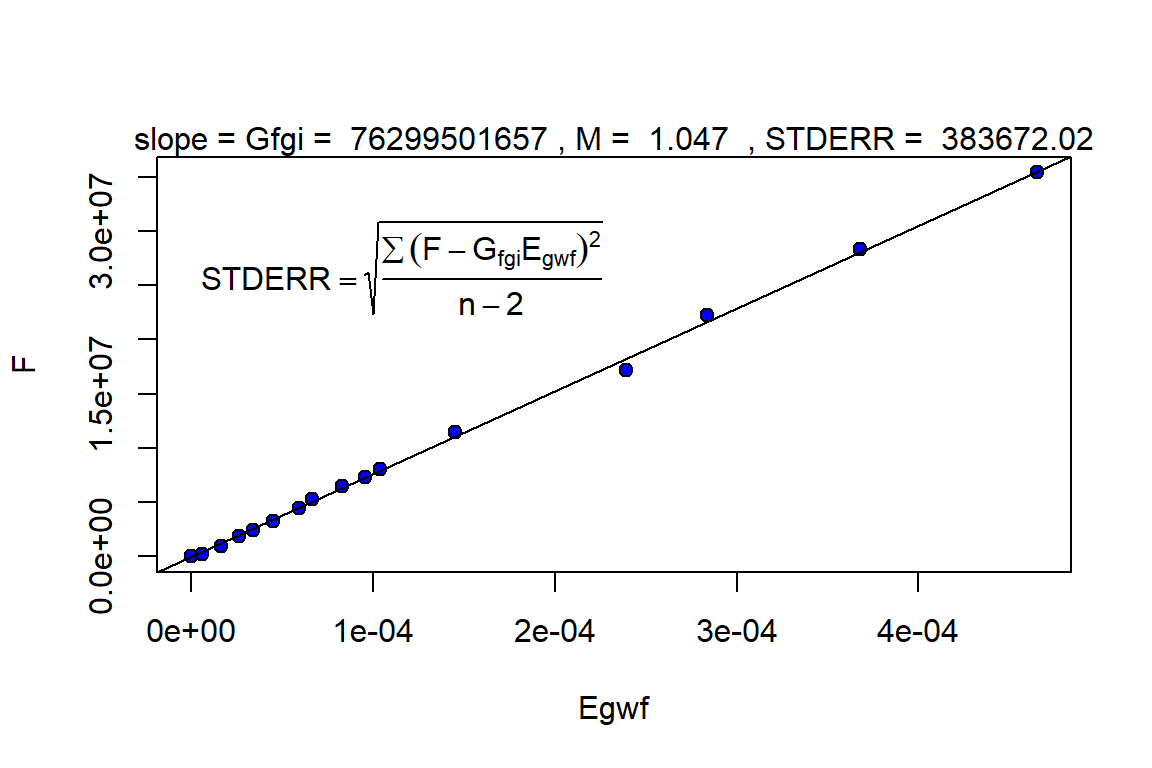
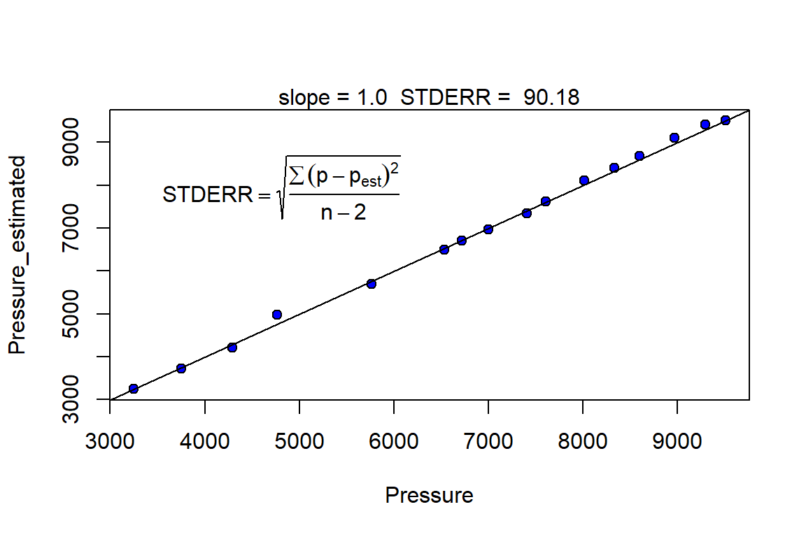
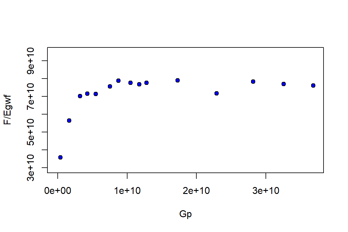
library(Rmbal)
library(Rrelperm)
library(pracma)
library(minpack.lm)
library(ggplot2)
library(dplyr)
library(magrittr)

# Anderson "L" gas reservoir

p_pvt <- c(9507, 9292, 8970, 8595, 8332, 8009, 7603, 7406, 7002, 6721, 6535,
           5764, 4766, 4295, 3750, 3247)    # Psia

Bg <- c(1.44, 1.418, 1.387, 1.344, 1.316, 1.282, 1.239, 1.218, 1.176, 1.147,
        1.127, 1.048, 0.977, 0.928, 0.891, 0.854) * (266 + 459.67) / p_pvt /
  ((60 + 459.67) / 14.696) / 5.615          # RB/SCF

Bo <- rep(0, length(p_pvt))                 # RB/STB

Rv <- rep(0, length(p_pvt))                 # STB/SCF

Rs <- rep(1e8, length(p_pvt))               # SCF/STB

Bw <- 1.055 * exp(3e-6 * (p_pvt[1] - p_pvt))     # RB/STB

muo <- rep(0.5, length(p_pvt))              # cp

muw <- rep(0.25, length(p_pvt))             # cp

mug <- rep(0.015, length(p_pvt))            # cp

pvt_table <- data.frame(p = p_pvt, Bo = Bo, Rs = Rs, Rv = Rv, Bg = Bg,
                             Bw = Bw, muo = muo, mug = mug, muw = muw)

p <- p_pvt

Gp <- c(0, 392.5, 1642.2, 3225.8, 4260.3, 5503.5, 7538.1, 8749.2, 10509.3, 11758.9,
        12789.2, 17262.5, 22890.8, 28144.6, 32566.7, 36819.9) *  1e6  # SCF

Np <- Rv * Gp                                                         # STB

Wp <- rep(0, length.out = length(p))

We <- rep(0, length.out = length(p))

Wi <- rep(0, length.out = length(p))

wf <- rep(1, length.out = length(p))

mbal_optim_gas_lst <- mbal_optim_param_gas(input_unit = "Field", output_unit = "Field",
                                          unknown_param = "G_M", aquifer_model = NULL,
                                          G = NULL, phi = 0.22, swi = 0.35,
                                          Np = Np, Gp = Gp, Wp = Wp, Wi = Wi,
                                          We = We, pd = 0, p = p, pvt = pvt_table,
                                          M = NULL, cf = 3.2e-6, wf = wf, sgrw = 0.0)

time_lst <- mbal_time(c(0:15), "month")

# a number of plots will be automatically generated for quality check

optim_results <- mbal_optim_gas(mbal_optim_gas_lst, time_lst)
glimpse(optim_results)
#> List of 17
#>  $ input_unit : chr "Field"
#>  $ output_unit: chr "Field"
#>  $ G          : num 7.63e+10
#>  $ phi        : num 0.22
#>  $ swi        : num 0.35
#>  $ pd         : num 0
#>  $ p          : num [1:16] 9507 9292 8970 8595 8332 ...
#>  $ cf         : num [1:16] 3.2e-06 3.2e-06 3.2e-06 3.2e-06 3.2e-06 3.2e-06 3.2e-06 3.2e-06 3.2e-06 3.2e-06 ...
#>  $ M          : num 1.05
#>  $ pvt        :'data.frame': 16 obs. of  9 variables:
#>   ..$ p  : num [1:16] 9507 9292 8970 8595 8332 ...
#>   ..$ Bo : num [1:16] 0 0 0 0 0 0 0 0 0 0 ...
#>   ..$ Rs : num [1:16] 1e+08 1e+08 1e+08 1e+08 1e+08 1e+08 1e+08 1e+08 1e+08 1e+08 ...
#>   ..$ Rv : num [1:16] 0 0 0 0 0 0 0 0 0 0 ...
#>   ..$ Bg : num [1:16] 0.000554 0.000558 0.000565 0.000571 0.000577 ...
#>   ..$ Bw : num [1:16] 1.05 1.06 1.06 1.06 1.06 ...
#>   ..$ muo: num [1:16] 0.5 0.5 0.5 0.5 0.5 0.5 0.5 0.5 0.5 0.5 ...
#>   ..$ mug: num [1:16] 0.015 0.015 0.015 0.015 0.015 0.015 0.015 0.015 0.015 0.015 ...
#>   ..$ muw: num [1:16] 0.25 0.25 0.25 0.25 0.25 0.25 0.25 0.25 0.25 0.25 ...
#>  $ prod       :'data.frame': 16 obs. of  3 variables:
#>   ..$ Np: num [1:16] 0 0 0 0 0 0 0 0 0 0 ...
#>   ..$ Gp: num [1:16] 0.00 3.92e+08 1.64e+09 3.23e+09 4.26e+09 ...
#>   ..$ Wp: num [1:16] 0 0 0 0 0 0 0 0 0 0 ...
#>  $ inj        :'data.frame': 16 obs. of  1 variable:
#>   ..$ Wi: num [1:16] 0 0 0 0 0 0 0 0 0 0 ...
#>  $ We         : num [1:16] 0 0 0 0 0 0 0 0 0 0 ...
#>  $ aquifer    :List of 3
#>   ..$ input_unit : chr "Field"
#>   ..$ output_unit: chr "Field"
#>   ..$ We         : num [1:16] 0 0 0 0 0 0 0 0 0 0 ...
#>   ..- attr(*, "class")= chr [1:2] "NoA" "aquifer"
#>  $ wf         : num [1:16] 1 1 1 1 1 1 1 1 1 1 ...
#>  $ sgrw       : num 0
#>  $ p_est      : num [1:16] 9507 9407 9106 8678 8406 ...
#>  - attr(*, "class")= chr [1:2] "volumetric_gas" "mbal_gas"
Part II: Reservoir Performance
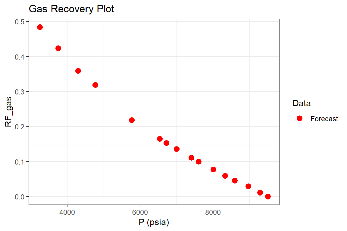
mbal_results <- mbal_perform_gas(optim_results, time_lst)

mbal_results
#>    P (psia) Eo (bbl/STB) Eg (bbl/SCF) Ew (bbl/STB) Ef (bbl/bbl) Egwf (bbl/SCF)
#> 1      9507            0 0.000000e+00 0.0000000000    0.0000000   0.000000e+00
#> 2      9292            0 4.155668e-06 0.0006806945    0.0006880   6.122769e-06
#> 3      8970            0 1.154615e-05 0.0017009748    0.0017184   1.646025e-05
#> 4      8595            0 1.791807e-05 0.0028904323    0.0029184   2.626564e-05
#> 5      8332            0 2.367540e-05 0.0037254372    0.0037600   3.443188e-05
#> 6      8009            0 3.144052e-05 0.0047518394    0.0047936   4.515649e-05
#> 7      7603            0 4.201038e-05 0.0060434035    0.0060928   5.944792e-05
#> 8      7406            0 4.748984e-05 0.0066706655    0.0067232   6.673380e-05
#> 9      7002            0 6.024781e-05 0.0079581904    0.0080160   8.319762e-05
#> 10     6721            0 7.014171e-05 0.0088546420    0.0089152   9.567015e-05
#> 11     6535            0 7.670890e-05 0.0094484385    0.0095104   1.039447e-04
#> 12     5764            0 1.109256e-04 0.0119133574    0.0119776   1.452424e-04
#> 13     4766            0 1.956269e-04 0.0151124827    0.0151712   2.391193e-04
#> 14     4295            0 2.360908e-04 0.0166256204    0.0166784   2.839172e-04
#> 15     3750            0 3.147957e-04 0.0183791614    0.0184224   3.676401e-04
#> 16     3247            0 4.076709e-04 0.0200001132    0.0200320   4.651495e-04
#>      Et (bbl)    F (bbl) We       Igd Inwd      Ifwd Iawd Itot     RF_oil
#> 1         0.0        0.0  0        NA   NA        NA   NA   NA 0.00000000
#> 2    467164.3   218911.0  0 0.6787236    0 0.3212764    0    1 0.01097792
#> 3   1255909.0   928049.1  0 0.7014563    0 0.2985437    0    1 0.02912672
#> 4   2004055.5  1843536.5  0 0.6821865    0 0.3178135    0    1 0.04595934
#> 5   2627135.3  2459278.5  0 0.6876010    0 0.3123990    0    1 0.05964763
#> 6   3445417.7  3219657.0  0 0.6962569    0 0.3037431    0    1 0.07718796
#> 7   4535846.5  4489615.2  0 0.7066754    0 0.2933246    0    1 0.09981353
#> 8   5091755.6  5258874.8  0 0.7116310    0 0.2883690    0    1 0.11102515
#> 9   6347937.2  6450894.1  0 0.7241530    0 0.2758470    0    1 0.13553916
#> 10  7299584.6  7334273.9  0 0.7331619    0 0.2668381    0    1 0.15338610
#> 11  7930925.2  8060882.8  0 0.7379783    0 0.2620217    0    1 0.16491605
#> 12 11081923.3 11471016.6  0 0.7637271    0 0.2362729    0    1 0.21857235
#> 13 18244680.9 17149932.0  0 0.8181145    0 0.1818855    0    1 0.31916344
#> 14 21662737.3 22224950.1  0 0.8315481    0 0.1684519    0    1 0.35953893
#> 15 28050756.1 28280110.1  0 0.8562605    0 0.1437395    0    1 0.42336556
#> 16 35490676.1 35393139.9  0 0.8764299    0 0.1235701    0    1 0.48390051
#>        RF_gas SOg  SGg  SWg SOT  SGT  SWT qo (STB/day) qg (SCF/day)
#> 1  0.00000000   0 0.65 0.35   0 0.65 0.35            0            0
#> 2  0.01097792   0 0.65 0.35   0 0.65 0.35            0     12904108
#> 3  0.02912672   0 0.65 0.35   0 0.65 0.35            0     41086023
#> 4  0.04595934   0 0.65 0.35   0 0.65 0.35            0     52063556
#> 5  0.05964763   0 0.65 0.35   0 0.65 0.35            0     34010955
#> 6  0.07718796   0 0.65 0.35   0 0.65 0.35            0     40872324
#> 7  0.09981353   0 0.65 0.35   0 0.65 0.35            0     66890952
#> 8  0.11102515   0 0.65 0.35   0 0.65 0.35            0     39816982
#> 9  0.13553916   0 0.65 0.35   0 0.65 0.35            0     57866295
#> 10 0.15338610   0 0.65 0.35   0 0.65 0.35            0     41082735
#> 11 0.16491605   0 0.65 0.35   0 0.65 0.35            0     33872873
#> 12 0.21857235   0 0.65 0.35   0 0.65 0.35            0    147067381
#> 13 0.31916344   0 0.65 0.35   0 0.65 0.35            0    185039980
#> 14 0.35953893   0 0.65 0.35   0 0.65 0.35            0    172727652
#> 15 0.42336556   0 0.65 0.35   0 0.65 0.35            0    145384094
#> 16 0.48390051   0 0.65 0.35   0 0.65 0.35            0    139831218
#>    qw (STB/day) fo fw GOR (SCF/STB) kro/krg
#> 1             0  0  0           Inf       0
#> 2             0  0  0           Inf       0
#> 3             0  0  0           Inf       0
#> 4             0  0  0           Inf       0
#> 5             0  0  0           Inf       0
#> 6             0  0  0           Inf       0
#> 7             0  0  0           Inf       0
#> 8             0  0  0           Inf       0
#> 9             0  0  0           Inf       0
#> 10            0  0  0           Inf       0
#> 11            0  0  0           Inf       0
#> 12            0  0  0           Inf       0
#> 13            0  0  0           Inf       0
#> 14            0  0  0           Inf       0
#> 15            0  0  0           Inf       0
#> 16            0  0  0           Inf       0

p1 <- mbal_results %>% ggplot(aes(`P (psia)`, `RF_gas`, color = "Forecast")) +
  geom_point(size = 3) +
  scale_color_manual(name="Data", values=c("Forecast" = "red")) +
  ggtitle("Gas Recovery Plot") +
  theme_bw()

p1
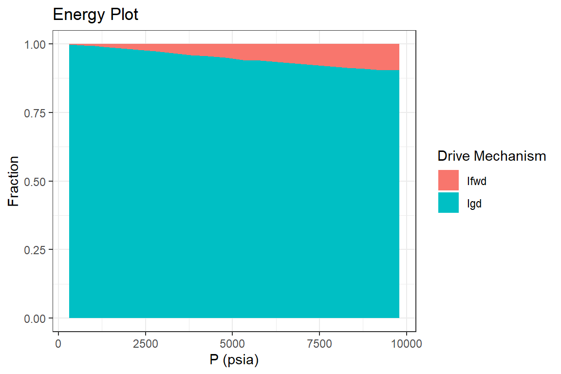
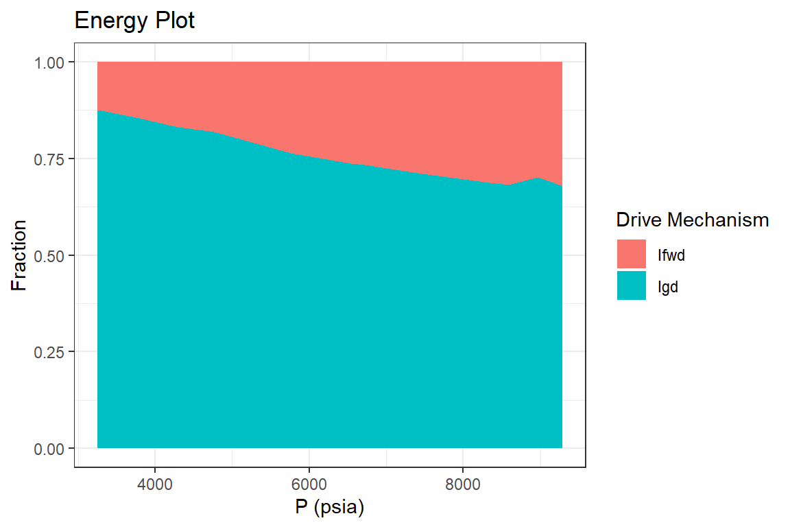
p2 <- mbal_results  %>%
  tidyr::pivot_longer(cols = c("Igd", "Ifwd"), names_to = "Drive Mechanism",
                      values_to = "Fraction", values_drop_na = TRUE) %>%
  ggplot(aes(`P (psia)`, Fraction, fill = `Drive Mechanism`)) +
  geom_area() +
  ggtitle("Energy Plot") +
  theme_bw()

p2
References
Fetkovich, M. J., Reese, D. E., & Whitson, C. H. (1998). Application of a General Material Balance for High-Pressure Gas Reservoirs (includes associated paper 51360). SPE Journal, 3(01), 3–13. https://doi.org/10.2118/22921-PA
Ikoku, Chi, U. (1984). Natural Gas Reservoir Engineering (p. 503). John Wiley & Sons, Ltd.
Pletcher, J. L. (2002). Improvements to Reservoir Material-Balance Methods. SPE Reservoir Evaluation & Engineering, 5(01), 49–59. https://doi.org/10.2118/75354-PA
Walsh, M. P., & Lake, L. W. (2003). A Generalized Approach to Primary Hydrocarbon Recovery (1st ed., p. 652; M. P. Walsh & L. W. Lake, Eds.). Retrieved from https://www.elsevier.com/books/a-generalized-approach-to-primary-hydrocarbon-recovery-of-petroleum-exploration-and-production/walsh/978-0-444-50683-2