Material Balance - Gas Condensate Reservoirs
GasCondensate.Rmd
Examples
Example 1: Lean Gas Condensate Reservoir (Walsh & Lake, 2003)
Part I: History Match
library(Rmbal)
library(Rrelperm)
library(pracma)
library(minpack.lm)
library(ggplot2)
library(dplyr)
#>
#> Attaching package: 'dplyr'
#> The following objects are masked from 'package:stats':
#>
#>     filter, lag
#> The following objects are masked from 'package:base':
#>
#>     intersect, setdiff, setequal, union
library(magrittr)
#>
#> Attaching package: 'magrittr'
#> The following objects are masked from 'package:pracma':
#>
#>     and, mod, or

p_pvt <- c(3700, 3650, 3400, 3100, 2800, 2500, 2200, 1900, 1600, 1300, 1000, 700,
           600, 400)

Bo <- c(10.057, 2.417, 2.192, 1.916, 1.736, 1.617, 1.504, 1.416, 1.326, 1.268, 1.205,
        1.149, 1.131, 1.093)

Rv <- c(84.11765, 84.11765, 70.5, 56.2, 46.5, 39.5, 33.8, 29.9, 27.3, 25.5, 25.9,
        28.3, 29.8, 33.5) / 1e6

Rs <- c(11566, 2378, 2010, 1569, 1272, 1067, 873, 719, 565, 461, 349, 249, 218, 141)

Bg <- c(0.87, 0.88, 0.92, 0.99, 1.08, 1.20, 1.35, 1.56, 1.85, 2.28, 2.95, 4.09,
        4.68, 6.53) / 1000

cw <- 3e-6

Bwi <- 10.05

Bw <- Bwi * exp(cw * (p_pvt[1] - p_pvt))

muo <- c(0.0612, 0.062, 0.1338, 0.1826, 0.2354, 0.3001, 0.3764, 0.4781, 0.6041,
         0.7746, 1.0295, 1.358, 1.855, 2.500)

mug <- c(0.0612, 0.062, 0.0554, 0.0436, 0.0368, 0.0308, 0.0261, 0.0222, 0.0191,
         0.0166, 0.0148, 0.0135, 0.0125, 0.0115)

muw <- rep(0.25, length(p_pvt))

pvt_table <- data.frame(p = p_pvt, Bo = Bo, Rs = Rs, Rv = Rv, Bg = Bg,
                               Bw = Bw, muo = muo, mug = mug, muw = muw)

p <- c(3700, 3650, 3400, 3100, 2800, 2500, 2200, 1900, 1600, 1300, 1000, 700,
           600)

We <- rep(0, length.out = length(p))

Np <- c(0, 28.6, 93, 231, 270, 379, 481, 517.2, 549, 580, 675, 755, 803) *1e3

Gp <- c(0, 0.34, 1.2, 3.3, 4.3, 6.6, 9.1, 10.5, 12, 12.8, 16.4, 19.1, 20.5) * 1e9

Wp <- rep(0, length.out = length(p))

Wi <- rep(0, length.out = length(p))

wf <- rep(1, length.out = length(p))

mbal_optim_gas_lst <- mbal_optim_param_gas(input_unit = "Field", output_unit = "Field",
                                          unknown_param = "G", aquifer_model = NULL,
                                          phi = 0.1, swi = 0.2, Np = Np,
                                          Gp = Gp, Wp = Wp, Wi = Wi, We = We,
                                          pd = 3650, p = p, pvt = pvt_table, M = 0,
                                          cf = 2e-6, wf = wf, sgrw = 0.15)

time_lst <- mbal_time(c(1:length(p)), "year")

# a number of plots will be automatically generated for quality check

optim_results <- mbal_optim_gas(mbal_optim_gas_lst, time_lst)
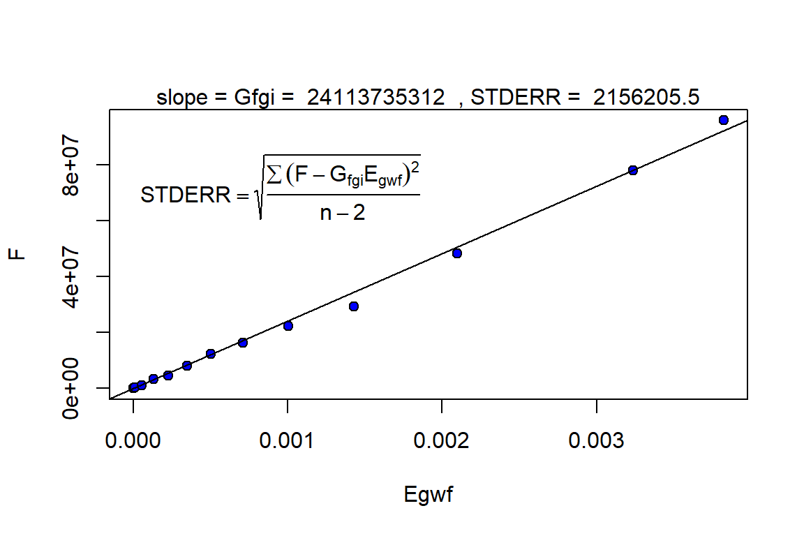
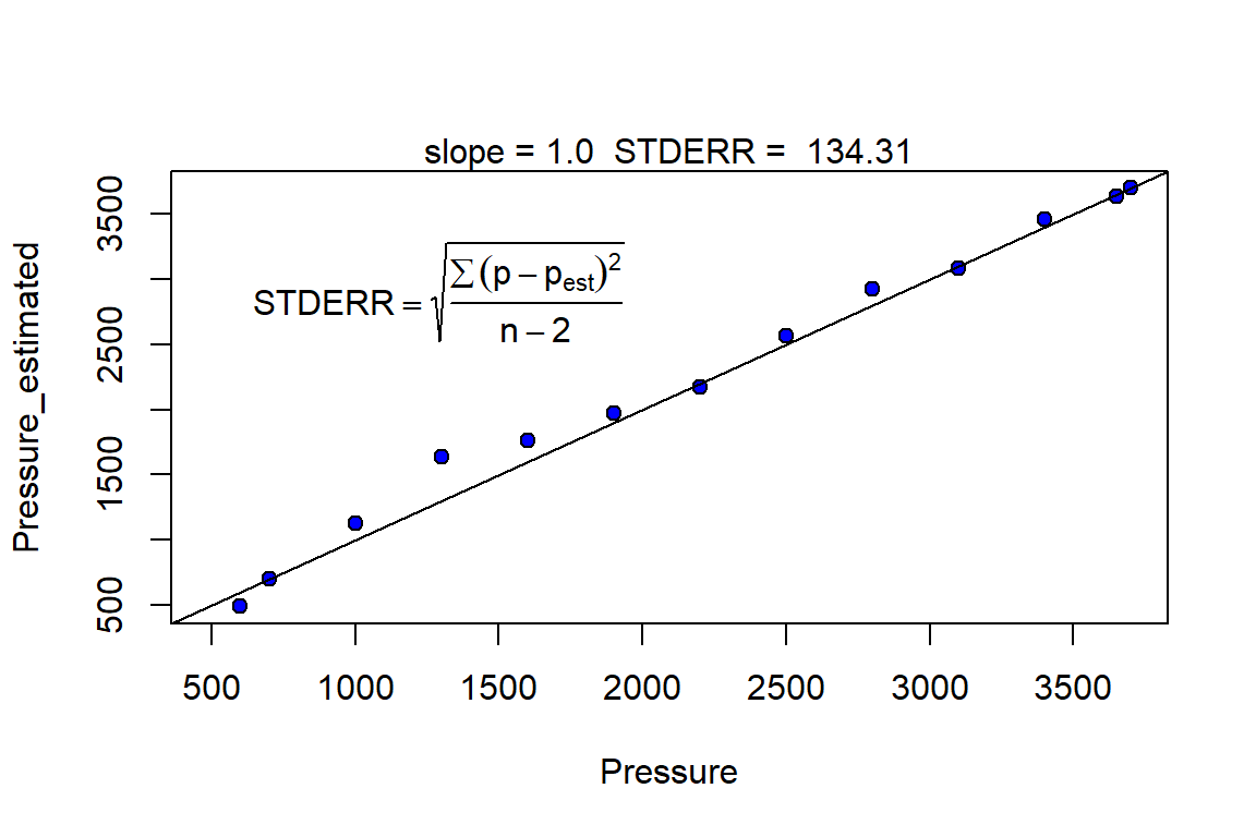
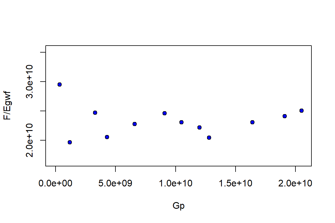
glimpse(optim_results)
#> List of 17
#>  $ input_unit : chr "Field"
#>  $ output_unit: chr "Field"
#>  $ G          : num 2.41e+10
#>  $ phi        : num 0.1
#>  $ swi        : num 0.2
#>  $ pd         : num 3650
#>  $ p          : num [1:13] 3700 3650 3400 3100 2800 2500 2200 1900 1600 1300 ...
#>  $ cf         : num [1:13] 2e-06 2e-06 2e-06 2e-06 2e-06 2e-06 2e-06 2e-06 2e-06 2e-06 ...
#>  $ M          : num 0
#>  $ pvt        :'data.frame': 14 obs. of  9 variables:
#>   ..$ p  : num [1:14] 3700 3650 3400 3100 2800 2500 2200 1900 1600 1300 ...
#>   ..$ Bo : num [1:14] 10.06 2.42 2.19 1.92 1.74 ...
#>   ..$ Rs : num [1:14] 11566 2378 2010 1569 1272 ...
#>   ..$ Rv : num [1:14] 8.41e-05 8.41e-05 7.05e-05 5.62e-05 4.65e-05 ...
#>   ..$ Bg : num [1:14] 0.00087 0.00088 0.00092 0.00099 0.00108 0.0012 0.00135 0.00156 0.00185 0.00228 ...
#>   ..$ Bw : num [1:14] 10.1 10.1 10.1 10.1 10.1 ...
#>   ..$ muo: num [1:14] 0.0612 0.062 0.1338 0.1826 0.2354 ...
#>   ..$ mug: num [1:14] 0.0612 0.062 0.0554 0.0436 0.0368 0.0308 0.0261 0.0222 0.0191 0.0166 ...
#>   ..$ muw: num [1:14] 0.25 0.25 0.25 0.25 0.25 0.25 0.25 0.25 0.25 0.25 ...
#>  $ prod       :'data.frame': 13 obs. of  3 variables:
#>   ..$ Np: num [1:13] 0 28600 93000 231000 270000 ...
#>   ..$ Gp: num [1:13] 0.0 3.4e+08 1.2e+09 3.3e+09 4.3e+09 ...
#>   ..$ Wp: num [1:13] 0 0 0 0 0 0 0 0 0 0 ...
#>  $ inj        :'data.frame': 13 obs. of  1 variable:
#>   ..$ Wi: num [1:13] 0 0 0 0 0 0 0 0 0 0 ...
#>  $ We         : num [1:13] 0 0 0 0 0 0 0 0 0 0 ...
#>  $ aquifer    :List of 3
#>   ..$ input_unit : chr "Field"
#>   ..$ output_unit: chr "Field"
#>   ..$ We         : num [1:13] 0 0 0 0 0 0 0 0 0 0 ...
#>   ..- attr(*, "class")= chr [1:2] "NoA" "aquifer"
#>  $ wf         : num [1:13] 1 1 1 1 1 1 1 1 1 1 ...
#>  $ sgrw       : num 0.15
#>  $ p_est      : num [1:13] 3700 3638 3459 3087 2928 ...
#>  - attr(*, "class")= chr [1:2] "volumetric_gas" "mbal_gas"
Part II: Reservoir Performance
mbal_results <- mbal_perform_gas(optim_results, time_lst)

mbal_results
#>    P (psia) Eo (bbl/STB) Eg (bbl/SCF) Ew (bbl/STB) Ef (bbl/bbl) Egwf (bbl/SCF)
#> 1      3700    0.0000000 0.000000e+00  0.000000000       0.0000   0.000000e+00
#> 2      3650    0.1320662 1.000000e-05  0.001507613       0.0001   1.014138e-05
#> 3      3400    0.6574474 5.543884e-05  0.009049071       0.0006   5.628718e-05
#> 4      3100    1.5325537 1.311046e-04  0.018106291       0.0012   1.328015e-04
#> 5      2800    2.6122256 2.244833e-04  0.027171665       0.0018   2.270288e-04
#> 6      2500    4.0130663 3.456791e-04  0.036245202       0.0024   3.490735e-04
#> 7      2200    5.7613484 4.968738e-04  0.045326909       0.0030   5.011172e-04
#> 8      1900    8.1827541 7.063101e-04  0.054416793       0.0036   7.114028e-04
#> 9      1600   11.5352122 9.962015e-04  0.063514862       0.0042   1.002144e-03
#> 10     1300   16.4682424 1.422867e-03  0.072621122       0.0048   1.429658e-03
#> 11     1000   24.1867133 2.090307e-03  0.081735582       0.0054   2.097949e-03
#> 12      700   37.3364090 3.227341e-03  0.090858249       0.0060   3.235832e-03
#> 13      600   44.1449393 3.816056e-03  0.093900963       0.0062   3.824830e-03
#>      Et (bbl)  F (bbl) We       Igd Inwd        Ifwd Iawd Itot     RF_oil
#> 1         0.0        0  0        NA   NA          NA   NA   NA 0.00000000
#> 2    244546.5   299200  0 0.9860593    0 0.013940655    0    1 0.01152429
#> 3   1357294.1  1107355  0 0.9849284    0 0.015071605    0    1 0.05619769
#> 4   3202339.9  3285114  0 0.9872226    0 0.012777361    0    1 0.11101389
#> 5   5474512.8  4670970  0 0.9887876    0 0.011212425    0    1 0.15600931
#> 6   8417466.8  7961572  0 0.9902759    0 0.009724057    0    1 0.19754688
#> 7  12083808.4 12343156  0 0.9915320    0 0.008467990    0    1 0.23215128
#> 8  17154579.3 16441143  0 0.9928414    0 0.007158640    0    1 0.26604491
#> 9  24165423.8 22263132  0 0.9940706    0 0.005929366    0    1 0.29378450
#> 10 34474400.5 29239665  0 0.9952495    0 0.004750542    0    1 0.33713256
#> 11 50589383.5 48424305  0 0.9963577    0 0.003642322    0    1 0.34765473
#> 12 78028003.4 78147206  0 0.9973758    0 0.002624158    0    1 0.37164849
#> 13 92230944.2 95961416  0 0.9977059    0 0.002294137    0    1 0.38049060
#>        RF_gas        SOg       SGg SWg        SOT       SGT SWT qo (STB/day)
#> 1  0.00000000 0.00000000 0.8000000 0.2 0.00000000 0.8000000 0.2      0.00000
#> 2  0.01152429 0.00000000 0.8000000 0.2 0.00000000 0.8000000 0.2     78.35616
#> 3  0.06099636 0.03081968 0.7691803 0.2 0.03081968 0.7691803 0.2    176.43836
#> 4  0.13340325 0.05019541 0.7498046 0.2 0.05019541 0.7498046 0.2    378.08219
#> 5  0.20899811 0.05785919 0.7421408 0.2 0.05785919 0.7421408 0.2    106.84932
#> 6  0.28937568 0.06103382 0.7389662 0.2 0.06103382 0.7389662 0.2    298.63014
#> 7  0.36944903 0.06151868 0.7384813 0.2 0.06151868 0.7384813 0.2    279.45205
#> 8  0.45433152 0.06031277 0.7396872 0.2 0.06031277 0.7396872 0.2     99.17808
#> 9  0.54016310 0.05791260 0.7420874 0.2 0.05791260 0.7420874 0.2     87.12329
#> 10 0.62584935 0.05444033 0.7455597 0.2 0.05444033 0.7455597 0.2     84.93151
#> 11 0.71051843 0.05289869 0.7471013 0.2 0.05289869 0.7471013 0.2    260.27397
#> 12 0.79087148 0.04988085 0.7501191 0.2 0.04988085 0.7501191 0.2    219.17808
#> 13 0.81708903 0.04878615 0.7512138 0.2 0.04878615 0.7512138 0.2    131.50685
#>    qg (SCF/day) qw (STB/day)          fo fw GOR (SCF/STB) kro/krg
#> 1           0.0            0 0.000000000  0      11888.11       0
#> 2      931506.8            0 0.000000000  0      11888.11       0
#> 3     2356164.4            0 0.022742723  0      13354.04       0
#> 4     5753424.7            0 0.033095319  0      15217.39       0
#> 5     2739726.0            0 0.037904222  0      25641.03       0
#> 6     6301369.9            0 0.027491083  0      21100.92       0
#> 7     6849315.1            0 0.023974224  0      24509.80       0
#> 8     3835616.4            0 0.018973378  0      38674.03       0
#> 9     4109589.0            0 0.008598187  0      47169.81       0
#> 10    2191780.8            0 0.021894547  0      25806.45       0
#> 11    9863013.7            0 0.000000000  0      37894.74       0
#> 12    7397260.3            0 0.000000000  0      33750.00       0
#> 13    3835616.4            0 0.000000000  0      29166.67       0
Part III: Reservoir Forecast
# Step I: generating a set of pseudo relative permeability curves using
# laboratory 'Kr' values

sg_lab <- c(0.05, 0.152, 0.248, 0.352, 0.448, 0.552, 0.65)

krg_lab <- c(0, 0.05, 0.09, 0.18, 0.3, 0.5, 1)

kro_lab <- c(1, 0.6, 0.35, 0.13, 0.04, 0.01, 0)

swcrit_lab <- 0.2

sgcrit_lab <- 0.05

sorgr_lab <- 0.15

fun_kr <- function(x, swcrit, sgcrit, sorg, sg, krg, kro) {

  kr_est <- Rrelperm::kr2p_gl(SWCON = swcrit, SOIRG = sorg, SORG = sorg,
                               SGCON = sgcrit, SGCRIT = sgcrit, KRGCL = 1,
                               KROGCG = 1, NG = x[1], NOG = x[2], NP = 101)

   krg_est_sub <- approx(x = kr_est[,1], y = kr_est[,3], xout = sg, rule = 2)$y

   kro_est_sub <- approx(x = kr_est[,1], y = kr_est[,4], xout = sg, rule = 2)$y

   error <- (krg - krg_est_sub) ^ 2 + (kro - kro_est_sub) ^ 2

   return(error)
}

par <- c(2, 2)

opt_results <- minpack.lm::nls.lm(par = par, fn = fun_kr, swcrit = swcrit_lab,
                                  sgcrit = sgcrit_lab, sorg = sorgr_lab, sg = sg_lab,
                                  krg = krg_lab, kro = kro_lab,
                                  lower = c(0.1,0.1), upper = c(10,10))

sol <- opt_results$par

sol
#> [1] 3.157478 2.740570

rel_perm <- as.data.frame(Rrelperm::kr2p_gl(SWCON = swcrit_lab, SOIRG = sorgr_lab,
                                            SORG = sorgr_lab, SGCON = sgcrit_lab,
                                            SGCRIT = sgcrit_lab, KRGCL = 1,
                                            KROGCG = 1, NG = sol[1], NOG = sol[2],
                                            NP = 101))

colnames(rel_perm) <- c("Sg", "Sl", "Krg", "Krog")

p_forecast <- p

wf_forecast <- wf

time_lst_forecast <- mbal_time(c(1:length(p_forecast)), "year")

forecast_lst <- mbal_forecast_param_gas(input_unit = "Field", output_unit = "Field",
                                        G = 2.41e10, phi = 0.1, swi = 0.2,
                                        pd = 3650, p = p_forecast, pvt = pvt_table,
                                        M = 0, cf = 2e-6, wf = wf_forecast,
                                        rel_perm = rel_perm)

glimpse(forecast_lst)
#> List of 12
#>  $ input_unit : chr "Field"
#>  $ output_unit: chr "Field"
#>  $ G          : num 2.41e+10
#>  $ phi        : num 0.1
#>  $ swi        : num 0.2
#>  $ pd         : num 3650
#>  $ p          : num [1:13] 3700 3650 3400 3100 2800 2500 2200 1900 1600 1300 ...
#>  $ cf         : num [1:13] 2e-06 2e-06 2e-06 2e-06 2e-06 2e-06 2e-06 2e-06 2e-06 2e-06 ...
#>  $ M          : num 0
#>  $ pvt        :'data.frame': 14 obs. of  9 variables:
#>   ..$ p  : num [1:14] 3700 3650 3400 3100 2800 2500 2200 1900 1600 1300 ...
#>   ..$ Bo : num [1:14] 10.06 2.42 2.19 1.92 1.74 ...
#>   ..$ Rs : num [1:14] 11566 2378 2010 1569 1272 ...
#>   ..$ Rv : num [1:14] 8.41e-05 8.41e-05 7.05e-05 5.62e-05 4.65e-05 ...
#>   ..$ Bg : num [1:14] 0.00087 0.00088 0.00092 0.00099 0.00108 0.0012 0.00135 0.00156 0.00185 0.00228 ...
#>   ..$ Bw : num [1:14] 10.1 10.1 10.1 10.1 10.1 ...
#>   ..$ muo: num [1:14] 0.0612 0.062 0.1338 0.1826 0.2354 ...
#>   ..$ mug: num [1:14] 0.0612 0.062 0.0554 0.0436 0.0368 0.0308 0.0261 0.0222 0.0191 0.0166 ...
#>   ..$ muw: num [1:14] 0.25 0.25 0.25 0.25 0.25 0.25 0.25 0.25 0.25 0.25 ...
#>  $ wf         : num [1:13] 1 1 1 1 1 1 1 1 1 1 ...
#>  $ rel_perm   :'data.frame': 101 obs. of  4 variables:
#>   ..$ Sg  : num [1:101] 0 0.01 0.02 0.03 0.04 0.05 0.06 0.07 0.08 0.09 ...
#>   ..$ Sl  : num [1:101] 1 0.99 0.98 0.97 0.96 0.95 0.94 0.93 0.92 0.91 ...
#>   ..$ Krg : num [1:101] 0 0 0 0 0 ...
#>   ..$ Krog: num [1:101] 1 1 1 1 1 ...
#>  - attr(*, "class")= chr [1:2] "volumetric_forecast_gas" "forecast_gas"

forecast_results <- mbal_forecast_gas(forecast_lst, time_lst_forecast)

forecast_results
#>    P (psia)        SOg       SGg SWg        SOT       SGT SWT GOR (SCF/STB)
#> 1      3700 0.00000000 0.8000000 0.2 0.00000000 0.8000000 0.2      11888.11
#> 2      3650 0.00000000 0.8000000 0.2 0.00000000 0.8000000 0.2      11888.11
#> 3      3400 0.03068653 0.7693135 0.2 0.03068653 0.7693135 0.2      14184.40
#> 4      3100 0.05013281 0.7498672 0.2 0.05013281 0.7498672 0.2      17793.59
#> 5      2800 0.05761899 0.7423810 0.2 0.05761899 0.7423810 0.2      21505.38
#> 6      2500 0.06091994 0.7390801 0.2 0.06091994 0.7390801 0.2      25316.46
#> 7      2200 0.06143071 0.7385693 0.2 0.06143071 0.7385693 0.2      29585.80
#> 8      1900 0.06042696 0.7395730 0.2 0.06042696 0.7395730 0.2      33444.82
#> 9      1600 0.05786851 0.7421315 0.2 0.05786851 0.7421315 0.2      36630.04
#> 10     1300 0.05603136 0.7439686 0.2 0.05603136 0.7439686 0.2      39215.69
#> 11     1000 0.05296314 0.7470369 0.2 0.05296314 0.7470369 0.2      38610.04
#> 12      700 0.04977272 0.7502273 0.2 0.04977272 0.7502273 0.2      35335.69
#> 13      600 0.04866108 0.7513389 0.2 0.04866108 0.7513389 0.2      33557.05
#>        RF_oil     RF_gas Liq_volume       Igd Inwd        Ifwd Iawd Itot
#> 1  0.00000000 0.00000000 0.00000000        NA   NA          NA   NA   NA
#> 2  0.01152429 0.01152429 0.00000000 0.9860593    0 0.013940655    0    1
#> 3  0.05685112 0.06097174 0.03758014 0.9849284    0 0.015071605    0    1
#> 4  0.11139035 0.13339023 0.05859826 0.9872226    0 0.012777361    0    1
#> 5  0.15766441 0.20894764 0.06341777 0.9887876    0 0.011212425    0    1
#> 6  0.19840889 0.28935420 0.06195818 0.9902759    0 0.009724057    0    1
#> 7  0.23287900 0.36943370 0.05704894 0.9915320    0 0.008467990    0    1
#> 8  0.26503067 0.45434807 0.04977378 0.9928414    0 0.007158640    0    1
#> 9  0.29420592 0.54015762 0.04100334 0.9940706    0 0.005929366    0    1
#> 10 0.32114068 0.62597917 0.03280231 0.9952495    0 0.004750542    0    1
#> 11 0.34697055 0.71052189 0.02391379 0.9963577    0 0.003642322    0    1
#> 12 0.37285555 0.79086821 0.01576379 0.9973758    0 0.002624158    0    1
#> 13 0.38190992 0.81708618 0.01319553 0.9977059    0 0.002294137    0    1

p1 <- forecast_results %>% ggplot(aes(`P (psia)`, SOg, color = "Forecast")) +
  geom_point(size = 3) +
  geom_point(data = mbal_results, aes(`P (psia)`, SOg, color = "Field"))+
  scale_color_manual(name="Data", values=c("Forecast" = "red", "Field" = "black")) +
  ggtitle("Condensate Saturation Plot") +
  theme_bw()

p1

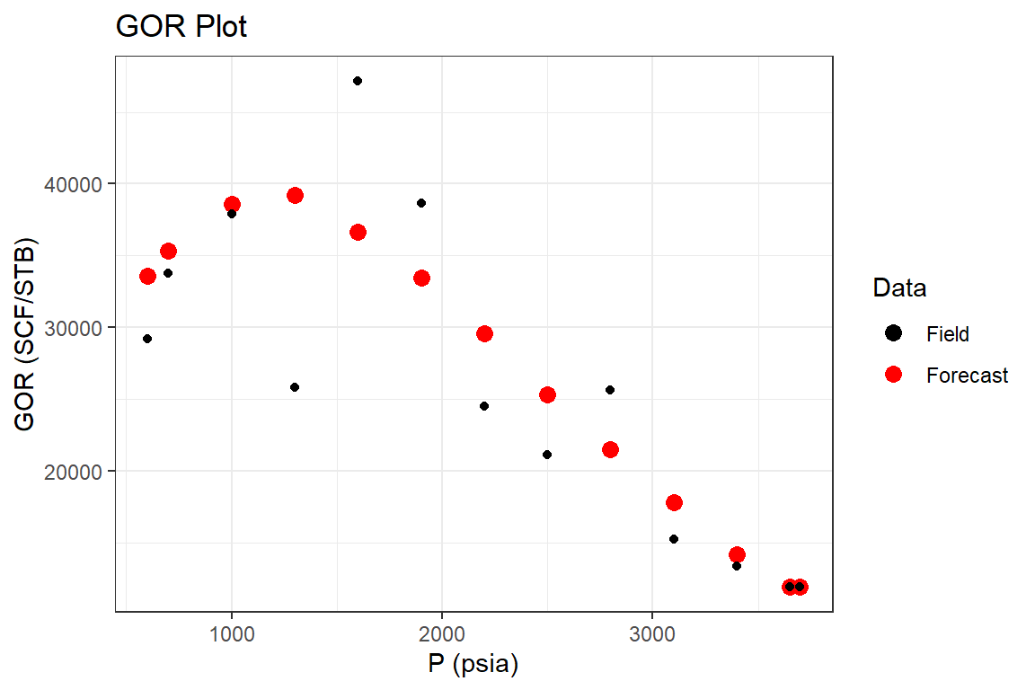
p2 <- forecast_results %>% ggplot(aes(`P (psia)`, `GOR (SCF/STB)`, color = "Forecast")) +
  geom_point(size = 3) +
  geom_point(data = mbal_results, aes(`P (psia)`, `GOR (SCF/STB)`, color = "Field")) +
  scale_color_manual(name="Data", values=c("Forecast" = "red", "Field" = "black")) +
  ggtitle("GOR Plot") +
  theme_bw()

p2
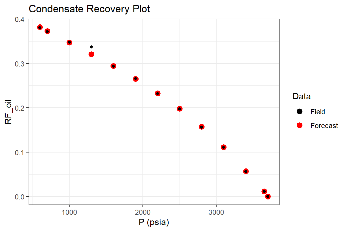
p3 <- forecast_results %>% ggplot(aes(`P (psia)`, `RF_oil`, color = "Forecast")) +
  geom_point(size = 3) +
  geom_point(data = mbal_results, aes(`P (psia)`, `RF_oil`, color = "Field")) +
  scale_color_manual(name="Data", values=c("Forecast" = "red", "Field" = "black")) +
  ggtitle("Condensate Recovery Plot") +
  theme_bw()

p3
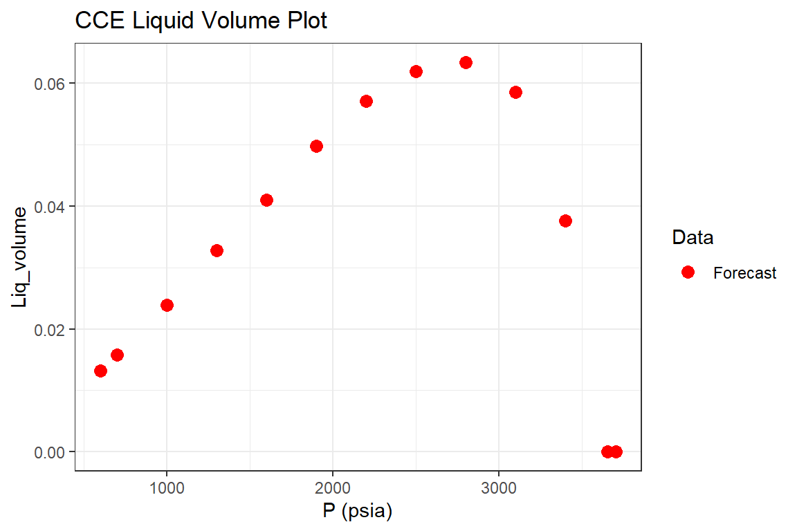
p4 <- forecast_results %>% ggplot(aes(`P (psia)`, `Liq_volume`, color = "Forecast")) +
  geom_point(size = 3) +
  scale_color_manual(name="Data", values=c("Forecast" = "red")) +
  ggtitle("CCE Liquid Volume Plot") +
  theme_bw()

p4
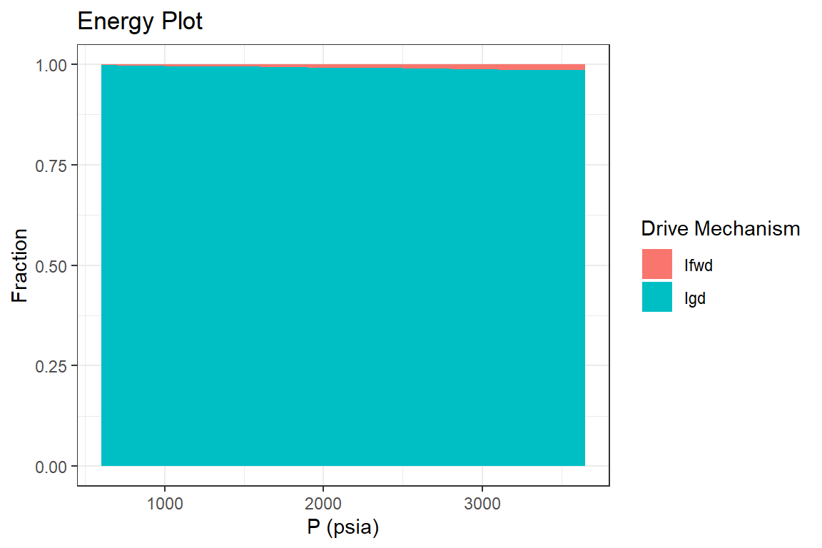
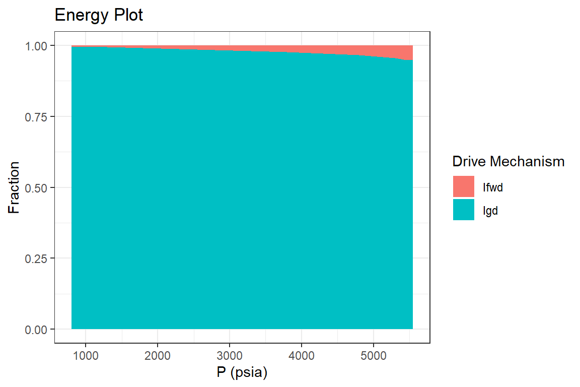
p5 <- forecast_results  %>%
  tidyr::pivot_longer(cols = c("Igd", "Ifwd"), names_to = "Drive Mechanism",
                      values_to = "Fraction", values_drop_na = TRUE) %>%
  ggplot(aes(`P (psia)`, Fraction, fill = `Drive Mechanism`)) +
  geom_area() +
  ggtitle("Energy Plot") +
  theme_bw()

p5
Example 2: Lean Gas Condensate Reservoir (Walsh, Ansah, & Raghavan, 1994)
Part I: Reservoir Forecast
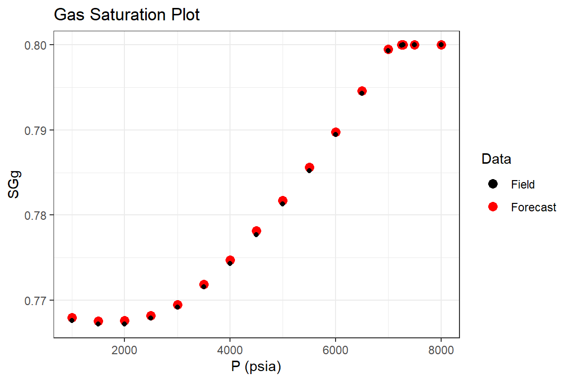
library(Rmbal)
library(Rrelperm)
library(pracma)
library(ggplot2)
library(dplyr)
library(magrittr)

p_pvt <- c(8000, 7500, 7280, 7250, 7000, 6500, 6000, 5500, 5000, 4500, 4000, 3500,
           3000,    2500,   2000,   1500,   1000) # psia

Bo <- c(12.732, 13.044, 13.192, 1.054, 1.041,   1.018,  1.002,  0.983,  0.965, 0.947,
        0.93,   0.913,  0.896,  0.877,  0.858,  0.839,  0.819) # RB/STB

Rs <- c(22527,  22527,  22527,  860,    819,    754,    704,    648,    593,    541, 490, 440,
        389,    336,    280,    228,    169) #SCF/STB

Bg <- c(0.565,  0.579,  0.586,  0.587,  0.595,  0.613,  0.634,  0.661, 0.694, 0.737,
        0.795,  0.817,  0.997,  1.178,  1.466,  1.963, 2.912) / 1000 # RB/SCF

Rv <- c(44.4,   44.4,   44.4,   44.3,   43.9,   40.3,   36.5,   32.9,   29.2,   25.4,   21.4,   17.6,
        13.7, 10.5, 7.9, 5.8,   4.4) / 1e6 # STB/SCF

cw <- 2e-6

Bwi <- 1.0

Bw <- Bwi * exp(cw * (p_pvt[1] - p_pvt))


muo <- c(0.049, 0.047,  0.046,  19.541, 20.965, 23.958, 26.338, 29.633, 33.319,
         37.401, 42.161,    47.465, 53.765, 61.887, 72.143, 83.478, 99.049)  # cp

muw <- rep(0.25, length(p_pvt))

mug <- c(0.049, 0.047,  0.046,  0.046,  0.0449, 0.042,  0.0393, 0.0366, 0.0339,
         0.0312,    0.0283, 0.0254, 0.0225, 0.0198, 0.0174, 0.0154, 0.014) # cp

pvt_table <- data.frame(p = p_pvt, Bo = Bo, Rs = Rs, Rv = Rv, Bg = Bg,
                               Bw = Bw, muo = muo, mug = mug, muw = muw)

p <- c(8000,    7500,   7280,   7250,   7000,   6500,   6000,   5500,   5000,   4500,   4000,   3500,
           3000,    2500,   2000,   1500,   1000) # psia

Gi <- rep(0, length.out = length(p))

wf <- rep(1, length.out = length(p))

# generating a set of pseudo relative permeability curves using
# laboratory 'Kr' values

sg_lab <- c(0.05, 0.152, 0.248, 0.352, 0.448, 0.552, 0.65)

krg_lab <- c(0, 0.05, 0.09, 0.18, 0.3, 0.5, 1)

kro_lab <- c(1, 0.6, 0.35, 0.13, 0.04, 0.01, 0)

swcrit_lab <- 0.2

sgcrit_lab <- 0.05

sorgr_lab <- 0.15

fun_kr <- function(x, swcrit, sgcrit, sorg, sg, krg, kro) {

  kr_est <- Rrelperm::kr2p_gl(SWCON = swcrit, SOIRG = sorg, SORG = sorg,
                               SGCON = sgcrit, SGCRIT = sgcrit, KRGCL = 1,
                               KROGCG = 1, NG = x[1], NOG = x[2], NP = 101)

   krg_est_sub <- approx(x = kr_est[,1], y = kr_est[,3], xout = sg, rule = 2)$y

   kro_est_sub <- approx(x = kr_est[,1], y = kr_est[,4], xout = sg, rule = 2)$y

   error <- (krg - krg_est_sub) ^ 2 + (kro - kro_est_sub) ^ 2

   return(error)
}

par <- c(2, 2)

opt_results <- minpack.lm::nls.lm(par = par, fn = fun_kr, swcrit = swcrit_lab,
                                  sgcrit = sgcrit_lab, sorg = sorgr_lab, sg = sg_lab,
                                  krg = krg_lab, kro = kro_lab,
                                  lower = c(0.1,0.1), upper = c(10,10))

sol <- opt_results$par

sol
#> [1] 3.157478 2.740570

rel_perm <- as.data.frame(Rrelperm::kr2p_gl(SWCON = swcrit_lab, SOIRG = sorgr_lab,
                                            SORG = sorgr_lab, SGCON = sgcrit_lab,
                                            SGCRIT = sgcrit_lab, KRGCL = 1,
                                            KROGCG = 1, NG = sol[1], NOG = sol[2],
                                            NP = 101))

colnames(rel_perm) <- c("Sg", "Sl", "Krg", "Krog")

p_forecast <- p

Gi_forecast <- Gi

wf_forecast <- wf

time_lst_forecast <- mbal_time(c(1:length(p_forecast)), "year")

forecast_lst <- mbal_forecast_param_gas(input_unit = "Field", output_unit = "Field",
                                        G = 1e6, phi = 0.1, swi = 0.2,
                                        pd = 7255, p = p_forecast, pvt = pvt_table,
                                        M = 0, cf = 2e-6, wf = wf_forecast,
                                        rel_perm = rel_perm)

forecast_results <- mbal_forecast_gas(forecast_lst, time_lst_forecast)

forecast_results
#>    P (psia)           SOg       SGg SWg           SOT       SGT SWT
#> 1      8000  0.000000e+00 0.8000000 0.2  0.000000e+00 0.8000000 0.2
#> 2      7500  0.000000e+00 0.8000000 0.2  0.000000e+00 0.8000000 0.2
#> 3      7280  0.000000e+00 0.8000000 0.2  0.000000e+00 0.8000000 0.2
#> 4      7250 -6.445867e-06 0.8000064 0.2 -6.445867e-06 0.8000064 0.2
#> 5      7000  5.302536e-04 0.7994697 0.2  5.302536e-04 0.7994697 0.2
#> 6      6500  5.429192e-03 0.7945708 0.2  5.429192e-03 0.7945708 0.2
#> 7      6000  1.023873e-02 0.7897613 0.2  1.023873e-02 0.7897613 0.2
#> 8      5500  1.437797e-02 0.7856220 0.2  1.437797e-02 0.7856220 0.2
#> 9      5000  1.826115e-02 0.7817389 0.2  1.826115e-02 0.7817389 0.2
#> 10     4500  2.185398e-02 0.7781460 0.2  2.185398e-02 0.7781460 0.2
#> 11     4000  2.525091e-02 0.7747491 0.2  2.525091e-02 0.7747491 0.2
#> 12     3500  2.809971e-02 0.7719003 0.2  2.809971e-02 0.7719003 0.2
#> 13     3000  3.051476e-02 0.7694852 0.2  3.051476e-02 0.7694852 0.2
#> 14     2500  3.181549e-02 0.7681845 0.2  3.181549e-02 0.7681845 0.2
#> 15     2000  3.238901e-02 0.7676110 0.2  3.238901e-02 0.7676110 0.2
#> 16     1500  3.243476e-02 0.7675652 0.2  3.243476e-02 0.7675652 0.2
#> 17     1000  3.201427e-02 0.7679857 0.2  3.201427e-02 0.7679857 0.2
#>    GOR (SCF/STB)     RF_oil     RF_gas   Liq_volume       Igd Inwd        Ifwd
#> 1       22522.52 0.00000000 0.00000000 0.0000000000        NA   NA          NA
#> 2       22522.52 0.02564347 0.02564347 0.0000000000 0.9429152    0 0.057084803
#> 3       22522.52 0.03791902 0.03791902 0.0000000000 0.9450713    0 0.054928735
#> 4       22573.36 0.03973609 0.03973814 0.0001866506 0.9454998    0 0.054500241
#> 5       22779.04 0.05363364 0.05373023 0.0009069775 0.9469934    0 0.053006646
#> 6       24813.90 0.08425990 0.08602965 0.0069953671 0.9519195    0 0.048080480
#> 7       27397.26 0.11423483 0.12068817 0.0127243519 0.9559001    0 0.044099860
#> 8       30395.14 0.14535094 0.16050244 0.0173040403 0.9602905    0 0.039709533
#> 9       34246.58 0.17580192 0.20404587 0.0212457921 0.9643350    0 0.035664961
#> 10      39370.08 0.20634170 0.25371497 0.0244042383 0.9685092    0 0.031490803
#> 11      46728.97 0.23638478 0.31100541 0.0267678152 0.9727908    0 0.027209242
#> 12      56818.18 0.24593832 0.33262872 0.0296404337 0.9722007    0 0.027799347
#> 13      72992.70 0.29008639 0.45412713 0.0273081939 0.9814057    0 0.018594281
#> 14      95238.10 0.31403419 0.53879463 0.0249801618 0.9853905    0 0.014609455
#> 15     126582.28 0.33373997 0.62969713 0.0211731296 0.9890246    0 0.010975366
#> 16     172413.79 0.34899766 0.72324482 0.0163934081 0.9922554    0 0.007744562
#> 17     227272.73 0.35976398 0.81315547 0.0112080103 0.9949920    0 0.005008048
#>    Iawd Itot
#> 1    NA   NA
#> 2     0    1
#> 3     0    1
#> 4     0    1
#> 5     0    1
#> 6     0    1
#> 7     0    1
#> 8     0    1
#> 9     0    1
#> 10    0    1
#> 11    0    1
#> 12    0    1
#> 13    0    1
#> 14    0    1
#> 15    0    1
#> 16    0    1
#> 17    0    1


reservoir_performance_table <- data.frame(p = p)

reservoir_performance_table$`RF_oil` <- c(0,    2.4,    3.5,    4.2,    5.8, 7.6,   10.4,
                                                13.8,   16.6,   20, 23.1,   25.9,   28.5,   30.8,
                                                32.7,   34.1,   35.2) / 100

reservoir_performance_table$`Sg` <- c(100,  100,    100,    99.99,  99.91,  99.29,  98.68,
                                      98.15,    97.66,  97.21,  96.79,  96.45,  96.15,
                                      95.99,    95.9,   95.9, 95.95) * 0.8 / 100


reservoir_performance_table$`GOR` <- c(22.53,   22.53, 22.53, 22.55, 22.78, 24.81,
                                       27.4, 30.4, 34.25,   39.37, 46.73, 56.82, 72.99,
                                       95.24, 126.58, 172.41, 227.27) * 1000 # SCF/STB


p1 <- forecast_results %>% ggplot(aes(`P (psia)`, SGg, color = "Forecast")) +
  geom_point(size = 3) +
  geom_point(data = reservoir_performance_table, aes(`p`, Sg, color = "Field"))+
  scale_color_manual(name="Data", values=c("Forecast" = "red", "Field" = "black")) +
  ggtitle("Gas Saturation Plot") +
  theme_bw()

p1
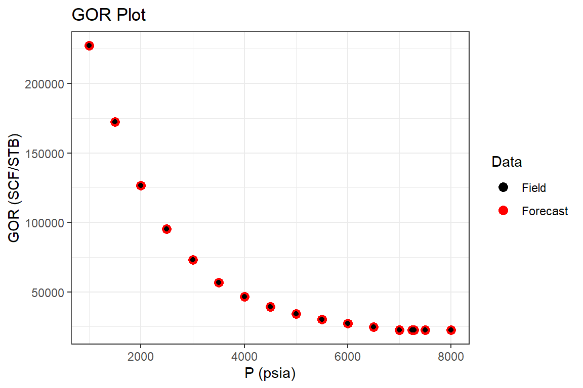
p2 <- forecast_results %>% ggplot(aes(`P (psia)`, `GOR (SCF/STB)`, color = "Forecast")) +
  geom_point(size = 3) +
  geom_point(data = reservoir_performance_table, aes(`p`, GOR, color = "Field"))+
  scale_color_manual(name="Data", values=c("Forecast" = "red", "Field" = "black")) +
  ggtitle("GOR Plot") +
  theme_bw()

p2
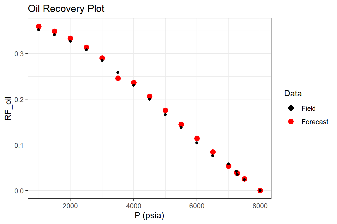
p3 <- forecast_results %>% ggplot(aes(`P (psia)`, `RF_oil`, color = "Forecast")) +
  geom_point(size = 3) +
  geom_point(data = reservoir_performance_table, aes(`p`, RF_oil, color = "Field"))+
  scale_color_manual(name="Data", values=c("Forecast" = "red", "Field" = "black")) +
  ggtitle("Oil Recovery Plot") +
  theme_bw()

p3
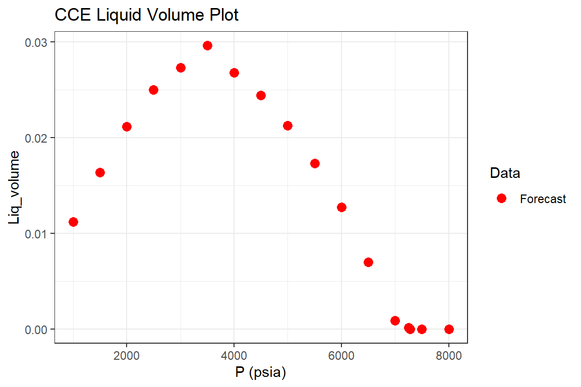
p4 <- forecast_results %>% ggplot(aes(`P (psia)`, `Liq_volume`, color = "Forecast")) +
  geom_point(size = 3) +
  scale_color_manual(name="Data", values=c("Forecast" = "red")) +
  ggtitle("CCE Liquid Volume Plot") +
  theme_bw()

p4
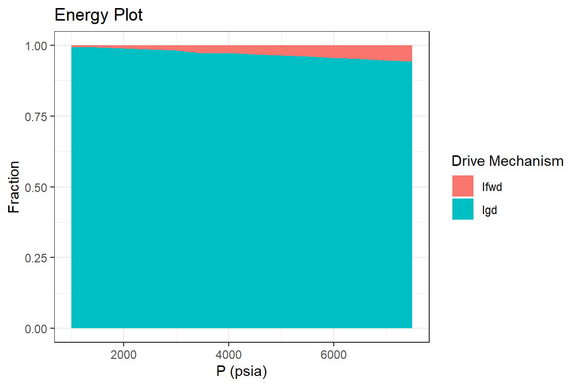
p5 <- forecast_results  %>%
  tidyr::pivot_longer(cols = c("Igd", "Ifwd"), names_to = "Drive Mechanism",
                      values_to = "Fraction", values_drop_na = TRUE) %>%
  ggplot(aes(`P (psia)`, Fraction, fill = `Drive Mechanism`)) +
  geom_area() +
  ggtitle("Energy Plot") +
  theme_bw()

p5
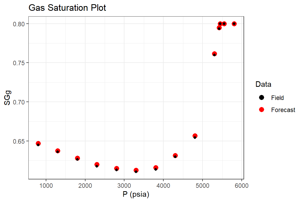
Example 3: Rich Gas Condensate Reservoir (Walsh et al., 1994)
Part I: Reservoir Forecast
library(Rmbal)
library(Rrelperm)
library(pracma)
library(ggplot2)
library(dplyr)
library(magrittr)

p_pvt <- c(5800,    5550,   5450,   5420,   5300,   4800,   4300,   3800,   3300,   2800,   2300,
           1800,    1300,   800) # psia

Bo <- c(4.382,  4.441,  4.468,  2.378,  2.366,  2.032,  1.828,  1.674,  1.554,
        1.448,  1.36,   1.279,  1.2,    1.131) # RB/STB

Rs <- c(6042,   6042,   6042,   2795,   2750,   2128,   1730,   1422,   1177,   960,    776,    607,
        443,    293) #SCF/STB

Bg <- c(0.725,  0.735,  0.739,  0.74,   0.743,  0.758,  0.794,  0.854,  0.947,
        1.09,   1.313,  1.677,  2.316,  3.695) / 1000 # RB/SCF

Rv <- c(165.5,  165.5,  165.5,  164.2,  156.6,  114,    89, 65.2,   48.3,   35, 25,
        19, 15, 13.5) / 1e6 # STB/SCF

cw <- 2e-6

Bwi <- 1.0

Bw <- Bwi * exp(cw * (p_pvt[1] - p_pvt))


muo <- c(0.0612,    0.062,  0.0587, 0.135,  0.1338, 0.1826, 0.2354, 0.3001, 0.3764,
         0.4781,    0.6041, 0.7746, 1.0295, 1.358)  # cp

muw <- rep(0.25, length(p_pvt))

mug <- c(0.0612,    0.062,  0.0587, 0.0581, 0.0554, 0.0436, 0.0368, 0.0308, 0.0261,
         0.0222,    0.0191, 0.0166, 0.0148, 0.0135) # cp

pvt_table <- data.frame(p = p_pvt, Bo = Bo, Rs = Rs, Rv = Rv, Bg = Bg,
                               Bw = Bw, muo = muo, mug = mug, muw = muw)

p <- c(5800,    5550,   5450,   5420,   5300,   4800,   4300,   3800,   3300,   2800,   2300,
           1800,    1300,   800) # psia

Gi <- rep(0, length.out = length(p))

wf <- rep(1, length.out = length(p))

# generating a set of pseudo relative permeability curves using
# laboratory 'Kr' values

sg_lab <- c(0.05, 0.152, 0.248, 0.352, 0.448, 0.552, 0.65)

krg_lab <- c(0, 0.05, 0.09, 0.18, 0.3, 0.5, 1)

kro_lab <- c(1, 0.6, 0.35, 0.13, 0.04, 0.01, 0)

swcrit_lab <- 0.2

sgcrit_lab <- 0.05

sorgr_lab <- 0.15

fun_kr <- function(x, swcrit, sgcrit, sorg, sg, krg, kro) {

  kr_est <- Rrelperm::kr2p_gl(SWCON = swcrit, SOIRG = sorg, SORG = sorg,
                               SGCON = sgcrit, SGCRIT = sgcrit, KRGCL = 1,
                               KROGCG = 1, NG = x[1], NOG = x[2], NP = 101)

   krg_est_sub <- approx(x = kr_est[,1], y = kr_est[,3], xout = sg, rule = 2)$y

   kro_est_sub <- approx(x = kr_est[,1], y = kr_est[,4], xout = sg, rule = 2)$y

   error <- (krg - krg_est_sub) ^ 2 + (kro - kro_est_sub) ^ 2

   return(error)
}

par <- c(2, 2)

opt_results <- minpack.lm::nls.lm(par = par, fn = fun_kr, swcrit = swcrit_lab,
                                  sgcrit = sgcrit_lab, sorg = sorgr_lab, sg = sg_lab,
                                  krg = krg_lab, kro = kro_lab,
                                  lower = c(0.1,0.1), upper = c(10,10))

sol <- opt_results$par

sol
#> [1] 3.157478 2.740570

rel_perm <- as.data.frame(Rrelperm::kr2p_gl(SWCON = swcrit_lab, SOIRG = sorgr_lab,
                                            SORG = sorgr_lab, SGCON = sgcrit_lab,
                                            SGCRIT = sgcrit_lab, KRGCL = 1,
                                            KROGCG = 1, NG = sol[1], NOG = sol[2],
                                            NP = 101))

colnames(rel_perm) <- c("Sg", "Sl", "Krg", "Krog")

p_forecast <- p

Gi_forecast <- Gi

wf_forecast <- wf

time_lst_forecast <- mbal_time(c(1:length(p_forecast)), "year")

forecast_lst <- mbal_forecast_param_gas(input_unit = "Field", output_unit = "Field",
                                        G = 1e6, phi = 0.1, swi = 0.2,
                                        pd = 5430, p = p_forecast, pvt = pvt_table,
                                        M = 0, cf = 2e-6, wf = wf_forecast,
                                        rel_perm = rel_perm)

forecast_results <- mbal_forecast_gas(forecast_lst, time_lst_forecast)

forecast_results
#>    P (psia)         SOg       SGg SWg         SOT       SGT SWT GOR (SCF/STB)
#> 1      5800 0.000000000 0.8000000 0.2 0.000000000 0.8000000 0.2      6042.296
#> 2      5550 0.000000000 0.8000000 0.2 0.000000000 0.8000000 0.2      6042.296
#> 3      5450 0.000000000 0.8000000 0.2 0.000000000 0.8000000 0.2      6042.296
#> 4      5420 0.005152288 0.7948477 0.2 0.005152288 0.7948477 0.2      6090.134
#> 5      5300 0.038538384 0.7614616 0.2 0.038538384 0.7614616 0.2      6385.696
#> 6      4800 0.143496208 0.6565038 0.2 0.143496208 0.6565038 0.2      8771.930
#> 7      4300 0.168505366 0.6314946 0.2 0.168505366 0.6314946 0.2     11235.330
#> 8      3800 0.183977117 0.6160229 0.2 0.183977117 0.6160229 0.2     15332.031
#> 9      3300 0.187431883 0.6125681 0.2 0.187431883 0.6125681 0.2     20693.172
#> 10     2800 0.185132689 0.6148673 0.2 0.185132689 0.6148673 0.2     28556.781
#> 11     2300 0.180121470 0.6198785 0.2 0.180121470 0.6198785 0.2     39984.461
#> 12     1800 0.172066360 0.6279336 0.2 0.172066360 0.6279336 0.2     52620.567
#> 13     1300 0.162517114 0.6374829 0.2 0.162517114 0.6374829 0.2     66662.406
#> 14      800 0.153317651 0.6466823 0.2 0.153317651 0.6466823 0.2     74073.272
#>        RF_oil     RF_gas Liq_volume       Igd Inwd        Ifwd Iawd Itot
#> 1  0.00000000 0.00000000 0.00000000        NA   NA          NA   NA   NA
#> 2  0.01434527 0.01434527 0.00000000 0.9484271    0 0.051572874    0    1
#> 3  0.01997469 0.01997469 0.00000000 0.9484263    0 0.051573690    0    1
#> 4  0.02236209 0.02237150 0.00771331 0.9501195    0 0.049880460    0    1
#> 5  0.03198528 0.03230067 0.04944218 0.9549330    0 0.045066956    0    1
#> 6  0.07264828 0.08203996 0.17567452 0.9658304    0 0.034169615    0    1
#> 7  0.10763210 0.13908121 0.19793410 0.9712101    0 0.028789884    0    1
#> 8  0.14065622 0.20995733 0.20452906 0.9763715    0 0.023628476    0    1
#> 9  0.16846524 0.29102297 0.19279839 0.9807127    0 0.019287285    0    1
#> 10 0.19178099 0.38362298 0.17088678 0.9846668    0 0.015333241    0    1
#> 11 0.21013894 0.48485147 0.14308242 0.9881815    0 0.011818547    0    1
#> 12 0.22436893 0.59186666 0.11048587 0.9912889    0 0.008711064    0    1
#> 13 0.23579468 0.70041590 0.07761736 0.9939804    0 0.006019611    0    1
#> 14 0.24476201 0.80834308 0.04661722 0.9963577    0 0.003642279    0    1

reservoir_performance_table <- data.frame(p = p)

reservoir_performance_table$`RF_oil` <- c(0,    1.3,    1.9,    2.1,    2.6,    7,  10.1,   13.3,
                                          16.2, 18.4,   20.2,   21.6,   22.8,   23.7) / 100

reservoir_performance_table$`Sg` <- c(100,  100,    100,    99.2,   95, 81.8,   78.7,   76.7,   76.3,
                                      76.6, 77.2,   78.3,   79.5,   80.6) * 0.8 / 100


reservoir_performance_table$`GOR` <- c(6.04,    6.04,   6.04,   6.09,   6.39,   8.77,   11.22,
                                       15.29,   20.62, 28.45, 39.82, 52.42, 66.48,
                                       73.99) * 1000 # SCF/STB


p1 <- forecast_results %>% ggplot(aes(`P (psia)`, SGg, color = "Forecast")) +
  geom_point(size = 3) +
  geom_point(data = reservoir_performance_table, aes(`p`, Sg, color = "Field"))+
  scale_color_manual(name="Data", values=c("Forecast" = "red", "Field" = "black")) +
  ggtitle("Gas Saturation Plot") +
  theme_bw()

p1
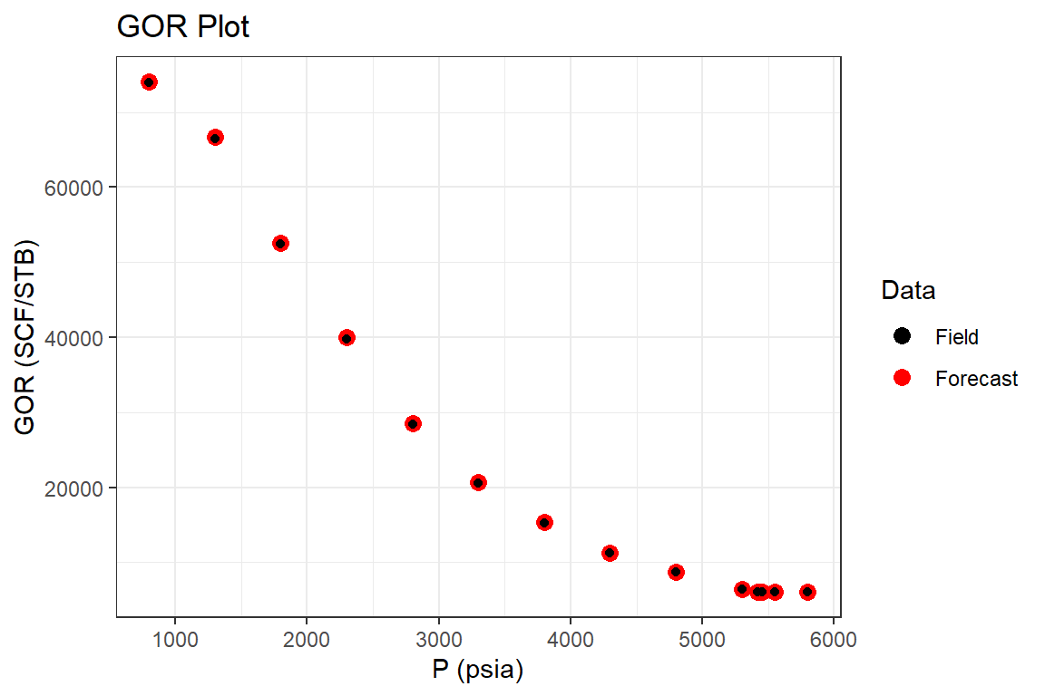
p2 <- forecast_results %>% ggplot(aes(`P (psia)`, `GOR (SCF/STB)`, color = "Forecast")) +
  geom_point(size = 3) +
  geom_point(data = reservoir_performance_table, aes(`p`, GOR, color = "Field"))+
  scale_color_manual(name="Data", values=c("Forecast" = "red", "Field" = "black")) +
  ggtitle("GOR Plot") +
  theme_bw()

p2
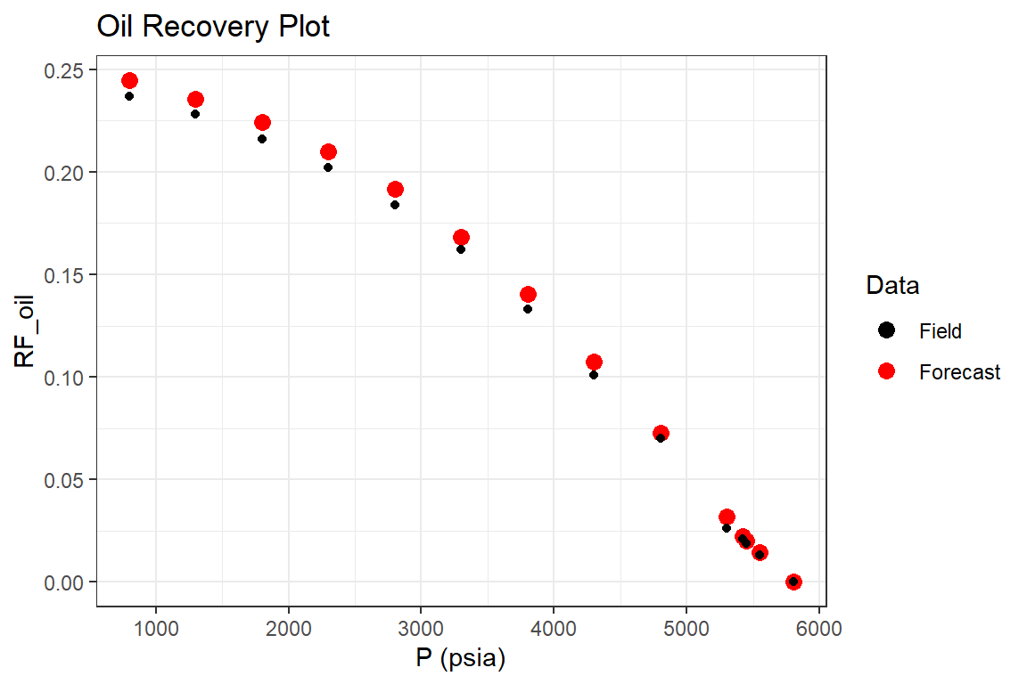
p3 <- forecast_results %>% ggplot(aes(`P (psia)`, `RF_oil`, color = "Forecast")) +
  geom_point(size = 3) +
  geom_point(data = reservoir_performance_table, aes(`p`, RF_oil, color = "Field"))+
  scale_color_manual(name="Data", values=c("Forecast" = "red", "Field" = "black")) +
  ggtitle("Oil Recovery Plot") +
  theme_bw()

p3
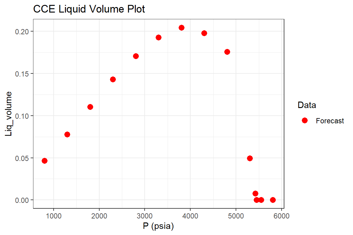
p4 <- forecast_results %>% ggplot(aes(`P (psia)`, `Liq_volume`, color = "Forecast")) +
  geom_point(size = 3) +
  scale_color_manual(name="Data", values=c("Forecast" = "red")) +
  ggtitle("CCE Liquid Volume Plot") +
  theme_bw()

p4
p5 <- forecast_results  %>%
  tidyr::pivot_longer(cols = c("Igd", "Ifwd"), names_to = "Drive Mechanism",
                      values_to = "Fraction", values_drop_na = TRUE) %>%
  ggplot(aes(`P (psia)`, Fraction, fill = `Drive Mechanism`)) +
  geom_area() +
  ggtitle("Energy Plot") +
  theme_bw()

p5
References
Walsh, M. P., Ansah, J., & Raghavan, R. (1994). New, generalized material balance as an equation of a straight line: Part 1- Applications to undersaturated, volumetric reservoirs. Proceedings of the Permian Basin Oil & Gas Recovery Conference, 549–564. https://doi.org/10.2118/27684-MS
Walsh, M. P., & Lake, L. W. (2003). A Generalized Approach to Primary Hydrocarbon Recovery (1st ed., p. 652; M. P. Walsh & L. W. Lake, Eds.). Retrieved from https://www.elsevier.com/books/a-generalized-approach-to-primary-hydrocarbon-recovery-of-petroleum-exploration-and-production/walsh/978-0-444-50683-2