Material Balance - Black Oil Reservoirs
BlackOil.Rmd
Examples
Example 1: Undersaturated Black Oil Reservoir (Ahmed & McKinney, 2004)
Part I: History Match
library(Rmbal)
library(Rrelperm)
library(pracma)
library(minpack.lm)
library(ggplot2)
library(dplyr)
#>
#> Attaching package: 'dplyr'
#> The following objects are masked from 'package:stats':
#>
#>     filter, lag
#> The following objects are masked from 'package:base':
#>
#>     intersect, setdiff, setequal, union
library(magrittr)
#>
#> Attaching package: 'magrittr'
#> The following objects are masked from 'package:pracma':
#>
#>     and, mod, or

 pvt_table_oil <- as.data.frame(Rpvt::pvt_oil("Field", "Field", "black_oil",
                                              "Standing", "Beggs_Robinson", 200,
                                              7150, 43, 0.7, c(0,0,0), pb = 4500,
                                              warning = "no"))

 colnames(pvt_table_oil) <- c("t", "p", "Rs", "Bo", "dens_o", "co", "muo", "Z",
                              "Bg", "dens_g", "cg", "mug", "m_p")

 pvt_table_water <- as.data.frame(Rpvt::pvt_water("Field", "Field", "water",
                                                  "Spivey", "Spivey", 200, 7150,
                                                  0, "no", "no"))

 colnames(pvt_table_water) <- c("t", "p", "Rsw", "Bw", "dens_w", "cw", "muw")

 pvt_table <- dplyr::left_join(pvt_table_oil, pvt_table_water, by = c("p", "t"))

 pvt_table$Rv <- rep(0, length.out = nrow(pvt_table))           # zero for black oil

 pvt_table <- pvt_table %>% dplyr::select(p, Bo, Rs, Rv, Bg, Bw, muo, mug, muw)

 p <- c(7150,6600,5800,4950,4500)

 We <- rep(0, length.out = length(p))

 Np <- c(0, 8.072, 22.549, 36.369, 43.473) * 1e6

 Rp <- c(0, rep(pvt_table$Rs[nrow(pvt_table)], 4))

 Wp <- rep(0, length.out = length(p))

 Wi <- rep(0, length.out = length(p))

 Gi <- rep(0, length.out = length(p))

 wf <- rep(1,length(p))

 mbal_optim_oil_lst <- mbal_optim_param_oil(input_unit = "Field", output_unit = "Field",
                                            unknown_param = "N", aquifer_model = NULL,
                                            m = 0, phi = 0.2, swi = 0.43, Np = Np,
                                            Rp = Rp, Wp = Wp, Gi = Gi, Wi = Wi, We = We,
                                            pb = 4500, p = p, pvt = pvt_table, cf = 4e-6,
                                            wf = wf, sorg = 0, sorw = 0)

 time_lst <- mbal_time(1:5, "year")

 # a number of plots will be automatically generated for quality check

 optim_results <- mbal_optim_oil(mbal_optim_oil_lst, time_lst)
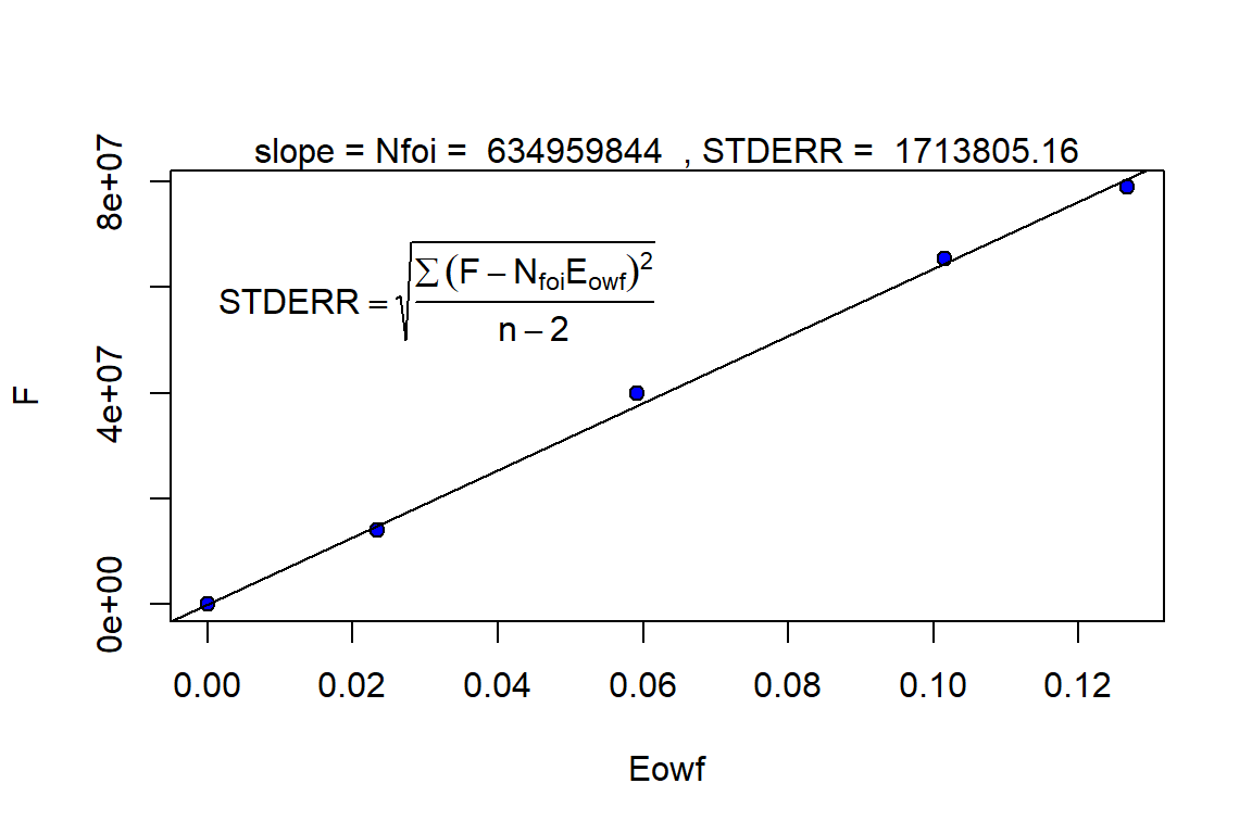
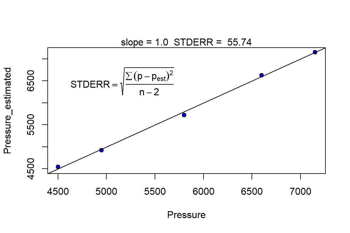
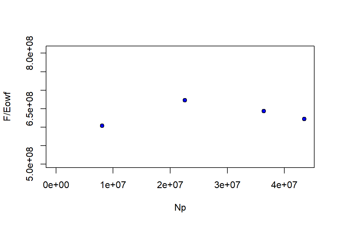
 glimpse(optim_results)
#> List of 18
#>  $ input_unit : chr "Field"
#>  $ output_unit: chr "Field"
#>  $ N          : num 6.35e+08
#>  $ m          : num 0
#>  $ phi        : num 0.2
#>  $ swi        : num 0.43
#>  $ pb         : num 4500
#>  $ p          : num [1:5] 7150 6600 5800 4950 4500
#>  $ cf         : num [1:5] 4e-06 4e-06 4e-06 4e-06 4e-06
#>  $ pvt        :'data.frame': 716 obs. of  9 variables:
#>   ..$ p  : num [1:716] 0 10 20 30 40 50 60 70 80 90 ...
#>   ..$ Bo : num [1:716] 1.07 1.07 1.07 1.07 1.07 ...
#>   ..$ Rs : num [1:716] 4.87 6.37 7.93 9.54 11.2 ...
#>   ..$ Rv : num [1:716] 0 0 0 0 0 0 0 0 0 0 ...
#>   ..$ Bg : num [1:716] 0.2257 0.1342 0.0954 0.074 0.0604 ...
#>   ..$ Bw : num [1:716] 1.04 1.04 1.04 1.04 1.04 ...
#>   ..$ muo: num [1:716] 1 0.993 0.985 0.978 0.97 ...
#>   ..$ mug: num [1:716] 0.0127 0.0127 0.0127 0.0127 0.0127 ...
#>   ..$ muw: num [1:716] 0.302 0.302 0.302 0.302 0.302 ...
#>  $ prod       :'data.frame': 5 obs. of  3 variables:
#>   ..$ Np: num [1:5] 0 8072000 22549000 36369000 43473000
#>   ..$ Rp: num [1:5] 1450 1450 1450 1450 1450
#>   ..$ Wp: num [1:5] 0 0 0 0 0
#>  $ inj        :'data.frame': 5 obs. of  2 variables:
#>   ..$ Gi: num [1:5] 0 0 0 0 0
#>   ..$ Wi: num [1:5] 0 0 0 0 0
#>  $ We         : num [1:5] 0 0 0 0 0
#>  $ aquifer    :List of 3
#>   ..$ input_unit : chr "Field"
#>   ..$ output_unit: chr "Field"
#>   ..$ We         : num [1:5] 0 0 0 0 0
#>   ..- attr(*, "class")= chr [1:2] "NoA" "aquifer"
#>  $ wf         : num [1:5] 1 1 1 1 1
#>  $ sorw       : num 0
#>  $ sorg       : num 0
#>  $ p_est      : num [1:5] 7150 6627 5723 4924 4545
#>  - attr(*, "class")= chr [1:2] "volumetric_oil" "mbal_oil"
Part II: Reservoir Performance
mbal_results <- mbal_perform_oil(optim_results, time_lst)

mbal_results
#>   P (psia) Eo (bbl/STB) Eg (bbl/SCF) Ew (bbl/STB) Ef (bbl/bbl) Eowf (bbl/STB)
#> 1     7150   0.00000000 0.000000e+00  0.000000000       0.0000     0.00000000
#> 2     6600   0.01458555 2.021415e-05  0.001602328       0.0022     0.02332055
#> 3     5800   0.03775399 5.761629e-05  0.003966834       0.0054     0.05923794
#> 4     4950   0.06642728 1.135771e-04  0.006524389       0.0088     0.10151519
#> 5     4500   0.08438586 1.539536e-04  0.007897814       0.0106     0.12670085
#>   Egwf (bbl/SCF) Et (bbl)  F (bbl) We Igd       Isd Inwd      Ifwd Iawd Itot
#> 1   0.000000e+00        0        0  0  NA        NA   NA        NA   NA   NA
#> 2   2.301691e-05 14807612 14077898  0   0 0.6254379    0 0.3745621    0    1
#> 3   6.450975e-05 37613713 39848802  0   0 0.6373278    0 0.3626722    0    1
#> 4   1.248356e-04 64458071 65314454  0   0 0.6543580    0 0.3456420    0    1
#> 5   1.675310e-04 80449954 78853117  0   0 0.6660244    0 0.3339756    0    1
#>       RF_oil     RF_gas  SOo SGo  SWo  SOT           SGT  SWT qo (STB/day)
#> 1 0.00000000 0.00000000 0.57   0 0.43 0.57 -5.551115e-17 0.43         0.00
#> 2 0.01337156 0.01337156 0.57   0 0.43 0.57 -5.551115e-17 0.43     22115.07
#> 3 0.03352061 0.03352061 0.57   0 0.43 0.57 -5.551115e-17 0.43     39663.01
#> 4 0.05652663 0.05652663 0.57   0 0.43 0.57 -5.551115e-17 0.43     37863.01
#> 5 0.06985223 0.06985223 0.57   0 0.43 0.57 -5.551115e-17 0.43     19463.01
#>   qg (SCF/day) qw (STB/day) fg fw GOR (SCF/STB) krg/kro
#> 1            0            0  0  0      1449.989       0
#> 2     32066603            0  0  0      1449.989       0
#> 3     57510928            0  0  0      1449.989       0
#> 4     54900948            0  0  0      1449.989       0
#> 5     28221153            0  0  0      1449.989       0
Part III: Reservoir Forecast
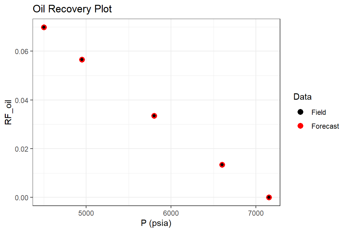
# gas saturation above the bubble point is zero, however the mbal_forecast_param_oil()
# requires a table of relative permeabilities as an input for the gas-oil system.
# Therefore, an arbitrary table is generated using the 'Rrelperm' package.
# The generated table does not impact the predictions above the bubble point.


rel_perm <- as.data.frame(Rrelperm::kr2p_gl(SWCON = 0.43, SOIRG = 0.15, SORG = 0.15,
                                            SGCON = 0.05, SGCRIT = 0.05, KRGCL = 1,
                                            KROGCG = 1, NG = 1.5, NOG = 1.0, NP = 101))

colnames(rel_perm) <- c("Sg", "Sl", "Krg", "Krog")

forecast_lst <- mbal_forecast_param_oil(input_unit = "Field", output_unit = "Field",
                                        N = 6.35e8, m = 0, phi = 0.1, swi = 0.43,
                                        Gi = Gi, pb = 4500, p = p, pvt = pvt_table,
                                        cf = 4e-6, wf = wf, sorg = 0, rel_perm = rel_perm)

glimpse(forecast_lst)
#> List of 14
#>  $ input_unit : chr "Field"
#>  $ output_unit: chr "Field"
#>  $ N          : num 6.35e+08
#>  $ m          : num 0
#>  $ phi        : num 0.1
#>  $ swi        : num 0.43
#>  $ pb         : num 4500
#>  $ p          : num [1:5] 7150 6600 5800 4950 4500
#>  $ cf         : num [1:5] 4e-06 4e-06 4e-06 4e-06 4e-06
#>  $ pvt        :'data.frame': 716 obs. of  9 variables:
#>   ..$ p  : num [1:716] 0 10 20 30 40 50 60 70 80 90 ...
#>   ..$ Bo : num [1:716] 1.07 1.07 1.07 1.07 1.07 ...
#>   ..$ Rs : num [1:716] 4.87 6.37 7.93 9.54 11.2 ...
#>   ..$ Rv : num [1:716] 0 0 0 0 0 0 0 0 0 0 ...
#>   ..$ Bg : num [1:716] 0.2257 0.1342 0.0954 0.074 0.0604 ...
#>   ..$ Bw : num [1:716] 1.04 1.04 1.04 1.04 1.04 ...
#>   ..$ muo: num [1:716] 1 0.993 0.985 0.978 0.97 ...
#>   ..$ mug: num [1:716] 0.0127 0.0127 0.0127 0.0127 0.0127 ...
#>   ..$ muw: num [1:716] 0.302 0.302 0.302 0.302 0.302 ...
#>  $ inj        :'data.frame': 5 obs. of  1 variable:
#>   ..$ Gi: num [1:5] 0 0 0 0 0
#>  $ wf         : num [1:5] 1 1 1 1 1
#>  $ sorg       : num 0
#>  $ rel_perm   :'data.frame': 101 obs. of  4 variables:
#>   ..$ Sg  : num [1:101] 0 0.01 0.02 0.03 0.04 0.05 0.06 0.07 0.08 0.09 ...
#>   ..$ Sl  : num [1:101] 1 0.99 0.98 0.97 0.96 0.95 0.94 0.93 0.92 0.91 ...
#>   ..$ Krg : num [1:101] 0 0 0 0 0 ...
#>   ..$ Krog: num [1:101] 1 1 1 1 1 ...
#>  - attr(*, "class")= chr [1:2] "volumetric_forecast_oil" "forecast_oil"

forecast_results <- mbal_forecast_oil(forecast_lst, time_lst)

forecast_results
#>   P (psia)  SOo SGo  SWo  SOT           SGT  SWT GOR (SCF/STB)     RF_oil
#> 1     7150 0.57   0 0.43 0.57 -5.551115e-17 0.43      1449.989 0.00000000
#> 2     6600 0.57   0 0.43 0.57 -5.551115e-17 0.43      1449.989 0.01337156
#> 3     5800 0.57   0 0.43 0.57 -5.551115e-17 0.43      1449.989 0.03352061
#> 4     4950 0.57   0 0.43 0.57 -5.551115e-17 0.43      1449.989 0.05652663
#> 5     4500 0.57   0 0.43 0.57 -5.551115e-17 0.43      1449.989 0.06985223
#>       RF_gas Liq_volume Igd       Isd Inwd      Ifwd Iawd Itot
#> 1 0.00000000          1  NA        NA   NA        NA   NA   NA
#> 2 0.01337156          1   0 0.6254379    0 0.3745621    0    1
#> 3 0.03352061          1   0 0.6373278    0 0.3626722    0    1
#> 4 0.05652663          1   0 0.6543580    0 0.3456420    0    1
#> 5 0.06985223          1   0 0.6660244    0 0.3339756    0    1

p1 <- forecast_results %>% ggplot(aes(`P (psia)`, `RF_oil`, color = "Forecast")) +
  geom_point(size = 3) +
  geom_point(data = mbal_results, aes(`P (psia)`, `RF_oil`, color = "Field"))+
  scale_color_manual(name="Data", values=c("Forecast" = "red", "Field" = "black")) +
  ggtitle("Oil Recovery Plot") +
  theme_bw()

p1
p2 <- forecast_results  %>%
  tidyr::pivot_longer(cols = c("Isd", "Ifwd"), names_to = "Drive Mechanism",
                      values_to = "Fraction", values_drop_na = TRUE) %>%
  ggplot(aes(`P (psia)`, Fraction, fill = `Drive Mechanism`)) +
  geom_area() +
  ggtitle("Energy Plot") +
  theme_bw()

p2
Example 2: Undersaturated Black Oil Reservoir (Ahmed & McKinney, 2004)
Part I: History Match
library(Rmbal)
library(Rrelperm)
library(pracma)
library(ggplot2)
library(dplyr)
library(magrittr)

 pvt_table_oil <- as.data.frame(Rpvt::pvt_oil("Field", "Field", "black_oil",
                                              "Standing", "Beggs_Robinson", 200,
                                              7150, 43, 0.7, c(0,0,0), pb = 4500,
                                              warning = "no"))

 colnames(pvt_table_oil) <- c("t", "p", "Rs", "Bo", "dens_o", "co", "muo", "Z",
                              "Bg", "dens_g", "cg", "mug", "m_p")

 pvt_table_water <- as.data.frame(Rpvt::pvt_water("Field", "Field", "water",
                                                  "Spivey", "Spivey", 200, 7150,
                                                  3e-6, "no", "no"))

 colnames(pvt_table_water) <- c("t", "p", "Rsw", "Bw", "dens_w", "cw", "muw")

 pvt_table <- dplyr::left_join(pvt_table_oil, pvt_table_water, by = c("p", "t"))

 pvt_table$Rv <- 0.0          # zero for black oil

 pvt_table <- pvt_table %>% dplyr::select(p, Bo, Rs, Rv, Bg, Bw, muo, mug, muw)

 p <- c(7150, 6600, 5800, 4950, 4500, 4350, 4060, 3840, 3600, 3480, 3260, 3100, 2940, 2800)

 We <- rep(0, length.out = length(p))

 Np <- c(0, 8.072, 22.549, 36.369, 43.473, 49.182, 58.383, 64.812, 69.562, 74.572,
         78.4, 81.275, 83.879, 86.401) * 1e6

 Rp <- c(0, rep(pvt_table$Rs[nrow(pvt_table)], 4), 1576, 1788, 1992, 2158, 2383, 2596, 2785, 2953, 3103)

 Wp <- rep(0, length.out = length(p))

 Wi <- rep(0, length.out = length(p))

 Gi <- rep(0, length.out = length(p))

 wf <- rep(1,length(p))

 mbal_optim_oil_lst <- mbal_optim_param_oil(input_unit = "Field", output_unit = "Field",
                                            unknown_param = "N", aquifer_model = NULL,
                                            m = 0, phi = 0.2, swi = 0.43, Np = Np,
                                            Rp = Rp, Wp = Wp, Gi = Gi, Wi = Wi, We = We,
                                            pb = 4500, p = p, pvt = pvt_table, cf = 4e-6,
                                            wf = wf, sorg = 0, sorw = 0)

 glimpse(mbal_optim_oil_lst)
#> List of 17
#>  $ input_unit : chr "Field"
#>  $ output_unit: chr "Field"
#>  $ N          : NULL
#>  $ m          : num 0
#>  $ phi        : num 0.2
#>  $ swi        : num 0.43
#>  $ pb         : num 4500
#>  $ p          : num [1:14] 7150 6600 5800 4950 4500 4350 4060 3840 3600 3480 ...
#>  $ cf         : num [1:14] 4e-06 4e-06 4e-06 4e-06 4e-06 4e-06 4e-06 4e-06 4e-06 4e-06 ...
#>  $ pvt        :'data.frame': 716 obs. of  9 variables:
#>   ..$ p  : num [1:716] 0 10 20 30 40 50 60 70 80 90 ...
#>   ..$ Bo : num [1:716] 1.07 1.07 1.07 1.07 1.07 ...
#>   ..$ Rs : num [1:716] 4.87 6.37 7.93 9.54 11.2 ...
#>   ..$ Rv : num [1:716] 0 0 0 0 0 0 0 0 0 0 ...
#>   ..$ Bg : num [1:716] 0.2257 0.1342 0.0954 0.074 0.0604 ...
#>   ..$ Bw : num [1:716] 1.04 1.04 1.04 1.04 1.04 ...
#>   ..$ muo: num [1:716] 1 0.993 0.985 0.978 0.97 ...
#>   ..$ mug: num [1:716] 0.0127 0.0127 0.0127 0.0127 0.0127 ...
#>   ..$ muw: num [1:716] 0.302 0.302 0.302 0.302 0.302 ...
#>  $ prod       :'data.frame': 14 obs. of  3 variables:
#>   ..$ Np: num [1:14] 0 8072000 22549000 36369000 43473000 ...
#>   ..$ Rp: num [1:14] 1450 1450 1450 1450 1450 ...
#>   ..$ Wp: num [1:14] 0 0 0 0 0 0 0 0 0 0 ...
#>  $ inj        :'data.frame': 14 obs. of  2 variables:
#>   ..$ Gi: num [1:14] 0 0 0 0 0 0 0 0 0 0 ...
#>   ..$ Wi: num [1:14] 0 0 0 0 0 0 0 0 0 0 ...
#>  $ We         : num [1:14] 0 0 0 0 0 0 0 0 0 0 ...
#>  $ aquifer    :List of 3
#>   ..$ input_unit : chr "Field"
#>   ..$ output_unit: chr "Field"
#>   ..$ We         : num [1:14] 0 0 0 0 0 0 0 0 0 0 ...
#>   ..- attr(*, "class")= chr [1:2] "NoA" "aquifer"
#>  $ wf         : num [1:14] 1 1 1 1 1 1 1 1 1 1 ...
#>  $ sorg       : num 0
#>  $ sorw       : num 0
#>  - attr(*, "class")= chr [1:2] "volumetric_optim_oil" "optimization_oil"


 time_lst <- mbal_time(1:14, "year")

 # a number of plots will be automatically generated for quality check

 optim_results <- mbal_optim_oil(mbal_optim_oil_lst, time_lst)
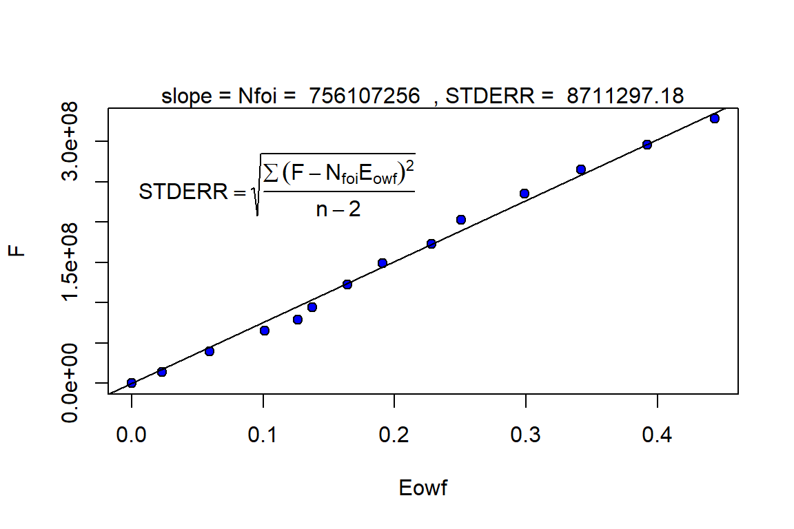
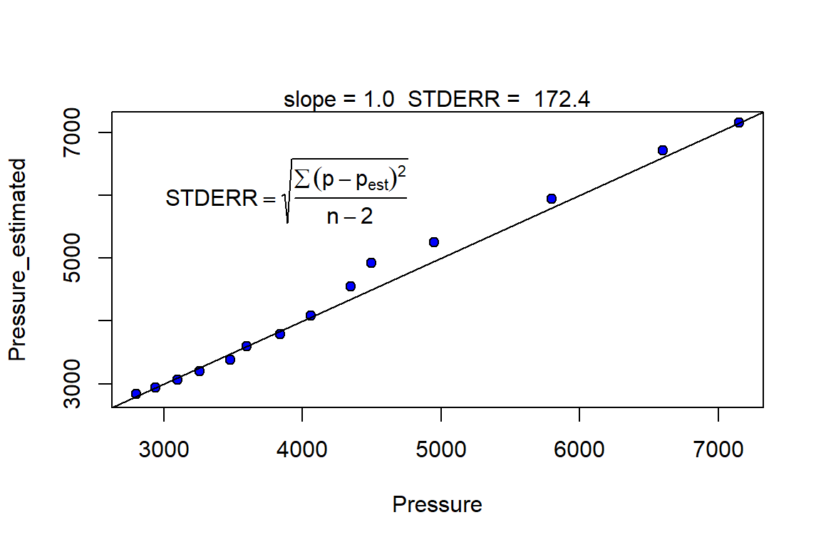
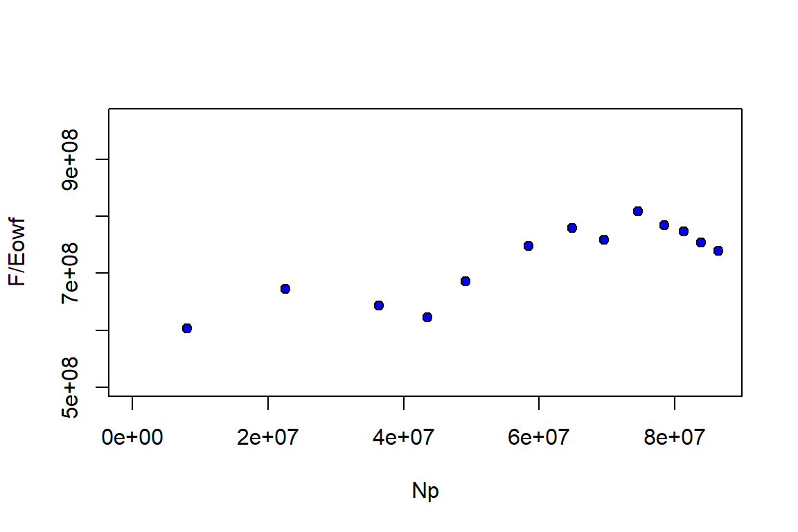
 glimpse(optim_results)
#> List of 18
#>  $ input_unit : chr "Field"
#>  $ output_unit: chr "Field"
#>  $ N          : num 7.56e+08
#>  $ m          : num 0
#>  $ phi        : num 0.2
#>  $ swi        : num 0.43
#>  $ pb         : num 4500
#>  $ p          : num [1:14] 7150 6600 5800 4950 4500 4350 4060 3840 3600 3480 ...
#>  $ cf         : num [1:14] 4e-06 4e-06 4e-06 4e-06 4e-06 4e-06 4e-06 4e-06 4e-06 4e-06 ...
#>  $ pvt        :'data.frame': 716 obs. of  9 variables:
#>   ..$ p  : num [1:716] 0 10 20 30 40 50 60 70 80 90 ...
#>   ..$ Bo : num [1:716] 1.07 1.07 1.07 1.07 1.07 ...
#>   ..$ Rs : num [1:716] 4.87 6.37 7.93 9.54 11.2 ...
#>   ..$ Rv : num [1:716] 0 0 0 0 0 0 0 0 0 0 ...
#>   ..$ Bg : num [1:716] 0.2257 0.1342 0.0954 0.074 0.0604 ...
#>   ..$ Bw : num [1:716] 1.04 1.04 1.04 1.04 1.04 ...
#>   ..$ muo: num [1:716] 1 0.993 0.985 0.978 0.97 ...
#>   ..$ mug: num [1:716] 0.0127 0.0127 0.0127 0.0127 0.0127 ...
#>   ..$ muw: num [1:716] 0.302 0.302 0.302 0.302 0.302 ...
#>  $ prod       :'data.frame': 14 obs. of  3 variables:
#>   ..$ Np: num [1:14] 0 8072000 22549000 36369000 43473000 ...
#>   ..$ Rp: num [1:14] 1450 1450 1450 1450 1450 ...
#>   ..$ Wp: num [1:14] 0 0 0 0 0 0 0 0 0 0 ...
#>  $ inj        :'data.frame': 14 obs. of  2 variables:
#>   ..$ Gi: num [1:14] 0 0 0 0 0 0 0 0 0 0 ...
#>   ..$ Wi: num [1:14] 0 0 0 0 0 0 0 0 0 0 ...
#>  $ We         : num [1:14] 0 0 0 0 0 0 0 0 0 0 ...
#>  $ aquifer    :List of 3
#>   ..$ input_unit : chr "Field"
#>   ..$ output_unit: chr "Field"
#>   ..$ We         : num [1:14] 0 0 0 0 0 0 0 0 0 0 ...
#>   ..- attr(*, "class")= chr [1:2] "NoA" "aquifer"
#>  $ wf         : num [1:14] 1 1 1 1 1 1 1 1 1 1 ...
#>  $ sorw       : num 0
#>  $ sorg       : num 0
#>  $ p_est      : num [1:14] 7150 6710 5944 5252 4916 ...
#>  - attr(*, "class")= chr [1:2] "volumetric_oil" "mbal_oil"
Part II: Reservoir Performance
mbal_results <- mbal_perform_oil(optim_results, time_lst)

mbal_results
#>    P (psia) Eo (bbl/STB) Eg (bbl/SCF) Ew (bbl/STB) Ef (bbl/bbl) Eowf (bbl/STB)
#> 1      7150   0.00000000 0.000000e+00  0.000000000      0.00000     0.00000000
#> 2      6600   0.01458555 2.021415e-05  0.001602328      0.00220     0.02332055
#> 3      5800   0.03775399 5.761629e-05  0.003966834      0.00540     0.05923794
#> 4      4950   0.06642728 1.135771e-04  0.006524389      0.00880     0.10151519
#> 5      4500   0.08438586 1.539536e-04  0.007897815      0.01060     0.12670085
#> 6      4350   0.09253750 1.697488e-04  0.008358672      0.01120     0.13726543
#> 7      4060   0.11460682 2.044881e-04  0.009254036      0.01236     0.16400540
#> 8      3840   0.13793039 2.353071e-04  0.009937161      0.01324     0.19087721
#> 9      3600   0.17134421 2.744243e-04  0.010686248      0.01420     0.22816680
#> 10     3480   0.19175249 2.965592e-04  0.011062315      0.01468     0.25051492
#> 11     3260   0.23686709 3.425341e-04  0.011754428      0.01556     0.29918932
#> 12     3100   0.27708164 3.811749e-04  0.012259960      0.01620     0.34199561
#> 13     2940   0.32482944 4.251195e-04  0.012767337      0.01684     0.39233753
#> 14     2800   0.37393276 4.687258e-04  0.013212818      0.01740     0.44371265
#>    Egwf (bbl/SCF)  Et (bbl)   F (bbl) We Igd       Isd Inwd      Ifwd Iawd Itot
#> 1    0.000000e+00         0         0  0  NA        NA   NA        NA   NA   NA
#> 2    2.301691e-05  17632836  14077898  0   0 0.6254379    0 0.3745621    0    1
#> 3    6.450975e-05  44790236  39848802  0   0 0.6373278    0 0.3626722    0    1
#> 4    1.248356e-04  76756374  65314454  0   0 0.6543580    0 0.3456420    0    1
#> 5    1.675310e-04  95799434  78853117  0   0 0.6660244    0 0.3339756    0    1
#> 6    1.841005e-04 103787389  94100389  0   0 0.6741501    0 0.3258499    0    1
#> 7    2.203384e-04 124005672 122648176  0   0 0.6987991    0 0.3012009    0    1
#> 8    2.522960e-04 144323642 148788859  0   0 0.7226132    0 0.2773868    0    1
#> 9    2.926567e-04 172518572 173069325  0   0 0.7509603    0 0.2490397    0    1
#> 10   3.154141e-04 189416148 202511466  0   0 0.7654334    0 0.2345666    0    1
#> 11   3.625311e-04 226219215 234793745  0   0 0.7916963    0 0.2083037    0    1
#> 12   4.020036e-04 258585364 264650747  0   0 0.8101906    0 0.1898094    0    1
#> 13   4.467805e-04 296649251 295866353  0   0 0.8279337    0 0.1720663    0    1
#> 14   4.911157e-04 335494356 327934206  0   0 0.8427363    0 0.1572637    0    1
#>        RF_oil     RF_gas       SOo        SGo  SWo       SOT           SGT  SWT
#> 1  0.00000000 0.00000000 0.5700000 0.00000000 0.43 0.5700000 -5.551115e-17 0.43
#> 2  0.01337156 0.01337156 0.5700000 0.00000000 0.43 0.5700000 -5.551115e-17 0.43
#> 3  0.03352061 0.03352061 0.5700000 0.00000000 0.43 0.5700000 -5.551115e-17 0.43
#> 4  0.05652663 0.05652663 0.5700000 0.00000000 0.43 0.5700000 -5.551115e-17 0.43
#> 5  0.06985223 0.06985223 0.5700000 0.00000000 0.43 0.5700000 -5.551115e-17 0.43
#> 6  0.07174241 0.07797717 0.5485941 0.02140590 0.43 0.5485941  2.140590e-02 0.43
#> 7  0.07806987 0.09626897 0.5221388 0.04786120 0.43 0.5221388  4.786120e-02 0.43
#> 8  0.08314556 0.11422568 0.5031687 0.06683135 0.43 0.5031687  6.683135e-02 0.43
#> 9  0.09170741 0.13648697 0.4847327 0.08526726 0.43 0.4847327  8.526726e-02 0.43
#> 10 0.09224860 0.15160696 0.4739048 0.09609520 0.43 0.4739048  9.609520e-02 0.43
#> 11 0.09990233 0.17886100 0.4582064 0.11179363 0.43 0.4582064  1.117936e-01 0.43
#> 12 0.10502783 0.20172741 0.4470325 0.12296749 0.43 0.4470325  1.229675e-01 0.43
#> 13 0.11122887 0.22652508 0.4362948 0.13370515 0.43 0.4362948  1.337052e-01 0.43
#> 14 0.11690521 0.25017907 0.4269536 0.14304640 0.43 0.4269536  1.430464e-01 0.43
#>    qo (STB/day) qg (SCF/day) qw (STB/day)        fg fw GOR (SCF/STB)    krg/kro
#> 1         0.000            0            0 0.0000000  0      1449.989 0.00000000
#> 2     22115.068     32066603            0 0.0000000  0      1449.989 0.00000000
#> 3     39663.014     57510928            0 0.0000000  0      1449.989 0.00000000
#> 4     37863.014     54900948            0 0.0000000  0      1449.989 0.00000000
#> 5     19463.014     28221153            0 0.0000000  0      1449.989 0.00000000
#> 6     15641.096     39658811            0 0.3915718  0      2535.552 0.03720636
#> 7     25208.219     73638279            0 0.4962545  0      2921.201 0.05384999
#> 8     17613.699     67716986            0 0.6162464  0      3844.564 0.08766729
#> 9     13013.699     57559704            0 0.6984738  0      4423.009 0.11107716
#> 10    13726.027     75589808            0 0.7294254  0      5507.042 0.14993374
#> 11    10487.671     70743353            0 0.8088469  0      6745.382 0.19733650
#> 12     7876.712     62532808            0 0.8407946  0      7938.948 0.24331382
#> 13     7134.247     58476197            0 0.8568752  0      8196.548 0.25807072
#> 14     6909.589     55911277            0 0.8617173  0      8091.838 0.26003598
Part III: Reservoir Forecast
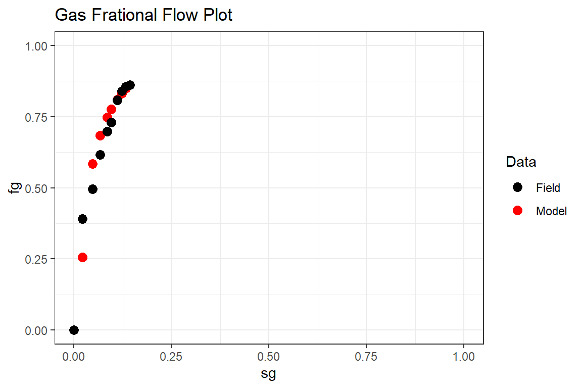
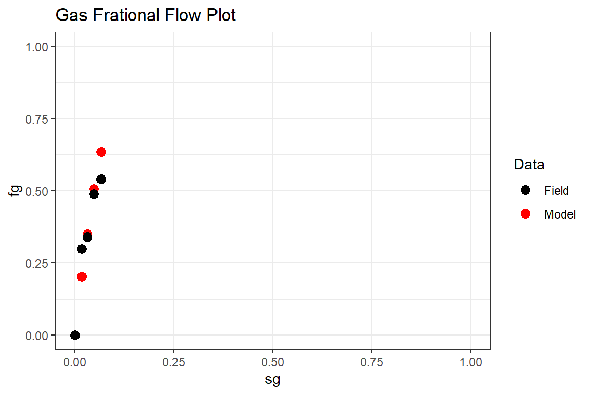
# Step I: generating a set of pseudo relative permeability curves by minimizing
# the difference between field and theoretical 'fg' values
# 'swcrit' and 'sgcrit' values are estimated from the 'mbal_results' data frame

fun_fg <- function(x, swcrit, sgcrit, muo, mug, sg, fg, krg_kro) {
  Kr_table <- Rrelperm::kr2p_gl(SWCON = swcrit, SOIRG = x[1], SORG = x[1],
                                            SGCON = sgcrit, SGCRIT = sgcrit, KRGCL = x[2],
                                            KROGCG = x[3], NG = x[4], NOG = x[5], NP = 101)
  l <- length(fg)
  krg_est_sub <- vector(length = l)
  kro_est_sub <- vector(length = l)
  krg_est_sub <- approx(x = Kr_table[,1], y = Kr_table[,3], xout = sg, rule = 2)$y
  kro_est_sub <- approx(x = Kr_table[,1], y = Kr_table[,4], xout = sg, rule = 2)$y
  fg_est <- (krg_est_sub / mug) / (krg_est_sub / mug + kro_est_sub / muo)
  krg_kro_est <- krg_est_sub / kro_est_sub
  error <- (fg - fg_est) ^ 2 + (krg_kro - krg_kro_est) ^ 2
  return(error)
}

swcrit <- 0.44
sgcrit <- 0.015
p <- mbal_results$`P (psia)`
sg <- mbal_results$SGo  # gas saturation in the oil leg
fg <- mbal_results$fg   # in-situ gas fractional flow
krg_kro <- mbal_results$`krg/kro`
muo <- approx(x = pvt_table$p, y = pvt_table$muo, xout = p, rule = 2)$y
mug <- approx(x = pvt_table$p, y = pvt_table$mug, xout = p, rule = 2)$y

par <- c(0.1, 1, 1, 2, 2)
lower = c(0, 0.1, 0.1, 0.1, 0.1)
upper = c(1 - swcrit - sgcrit, 1.0, 1.0, 10.0, 10.0)
opt_results <- minpack.lm::nls.lm(par = par, fn = fun_fg, swcrit = swcrit, sgcrit = sgcrit,
                                  muo = muo, mug = mug, sg = sg, fg = fg, krg_kro = krg_kro,
                                  lower = lower, upper = upper)

opt_results
#> Nonlinear regression via the Levenberg-Marquardt algorithm
#> parameter estimates: 0, 1, 1, 0.805733179825336, 0.1
#> residual sum-of-squares: 0.0006949
#> reason terminated: Relative error between `par' and the solution is at most `ptol'.

sol <- opt_results$par

sol
#> [1] 0.0000000 1.0000000 1.0000000 0.8057332 0.1000000

rel_perm <- as.data.frame(Rrelperm::kr2p_gl(SWCON = swcrit, SOIRG = sol[1], SORG = sol[1],
                                            SGCON = sgcrit, SGCRIT = sgcrit, KRGCL = sol[2],
                                            KROGCG = sol[3], NG = sol[4], NOG = sol[5],
                                            NP = 101))

colnames(rel_perm) <- c("Sg", "Sl", "Krg", "Krog")

krg_est <- approx(x = rel_perm[,1], y = rel_perm[,3], xout = sg, rule = 2)$y

kro_est <- approx(x = rel_perm[,1], y = rel_perm[,4], xout = sg, rule = 2)$y

fg_est <- (krg_est/ mug) / (krg_est / mug + kro_est / muo)

fg_df <- data.frame(Sg = sg)

fg_df$fg <- fg_est

p_fg <- fg_df %>% ggplot(aes(sg, fg, color = "Model")) +
  geom_point(size = 3) +
  geom_point(data = mbal_results, aes(SGo, fg, color = "Field"), size = 3)+
  xlim(c(0,1)) +
  ylim(c(0,1)) +
  scale_color_manual(name="Data", values=c("Model" = "red", "Field" = "black")) +
  ggtitle("Gas Frational Flow Plot") +
  theme_bw()

p_fg
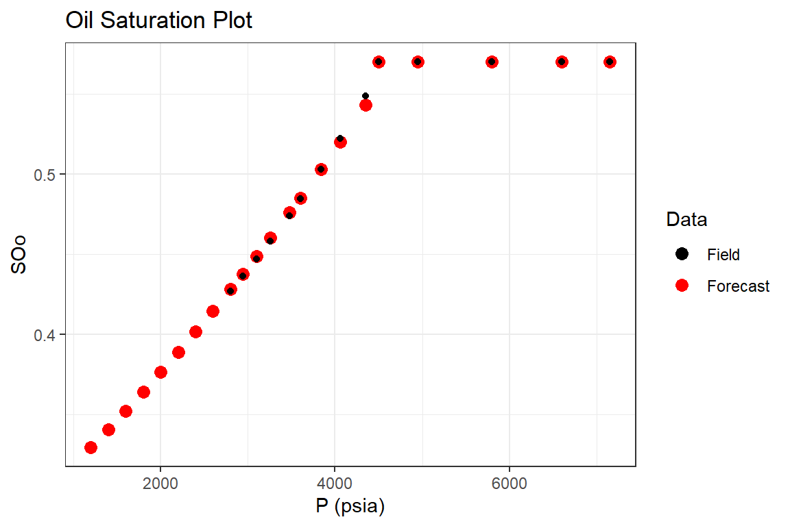
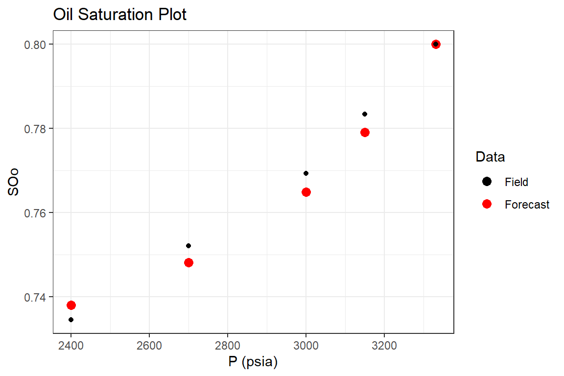
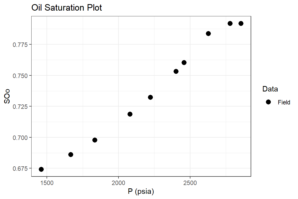
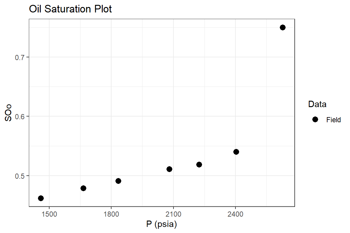
p_forecast <- c(p, 2600, 2400, 2200, 2000, 1800, 1600, 1400, 1200)

Gi_forecast <- c(Gi, 0, 0, 0, 0, 0, 0, 0, 0)

wf_forecast <- c(wf, 1, 1, 1, 1, 1, 1, 1, 1)

time_lst_forecast <-  mbal_time(1:22, "year")

forecast_lst <- mbal_forecast_param_oil(input_unit = "Field", output_unit = "Field",
                                        N = 6.35e8, m = 0, phi = 0.1, swi = 0.43,
                                        Gi = Gi_forecast, pb = 4500, p = p_forecast, pvt = pvt_table,
                                        cf = 4e-6, wf = wf_forecast, sorg = 0, rel_perm = rel_perm)

glimpse(forecast_lst)
#> List of 14
#>  $ input_unit : chr "Field"
#>  $ output_unit: chr "Field"
#>  $ N          : num 6.35e+08
#>  $ m          : num 0
#>  $ phi        : num 0.1
#>  $ swi        : num 0.43
#>  $ pb         : num 4500
#>  $ p          : num [1:22] 7150 6600 5800 4950 4500 4350 4060 3840 3600 3480 ...
#>  $ cf         : num [1:22] 4e-06 4e-06 4e-06 4e-06 4e-06 4e-06 4e-06 4e-06 4e-06 4e-06 ...
#>  $ pvt        :'data.frame': 716 obs. of  9 variables:
#>   ..$ p  : num [1:716] 0 10 20 30 40 50 60 70 80 90 ...
#>   ..$ Bo : num [1:716] 1.07 1.07 1.07 1.07 1.07 ...
#>   ..$ Rs : num [1:716] 4.87 6.37 7.93 9.54 11.2 ...
#>   ..$ Rv : num [1:716] 0 0 0 0 0 0 0 0 0 0 ...
#>   ..$ Bg : num [1:716] 0.2257 0.1342 0.0954 0.074 0.0604 ...
#>   ..$ Bw : num [1:716] 1.04 1.04 1.04 1.04 1.04 ...
#>   ..$ muo: num [1:716] 1 0.993 0.985 0.978 0.97 ...
#>   ..$ mug: num [1:716] 0.0127 0.0127 0.0127 0.0127 0.0127 ...
#>   ..$ muw: num [1:716] 0.302 0.302 0.302 0.302 0.302 ...
#>  $ inj        :'data.frame': 22 obs. of  1 variable:
#>   ..$ Gi: num [1:22] 0 0 0 0 0 0 0 0 0 0 ...
#>  $ wf         : num [1:22] 1 1 1 1 1 1 1 1 1 1 ...
#>  $ sorg       : num 0
#>  $ rel_perm   :'data.frame': 101 obs. of  4 variables:
#>   ..$ Sg  : num [1:101] 0 0.01 0.02 0.03 0.04 0.05 0.06 0.07 0.08 0.09 ...
#>   ..$ Sl  : num [1:101] 1 0.99 0.98 0.97 0.96 0.95 0.94 0.93 0.92 0.91 ...
#>   ..$ Krg : num [1:101] 0 0 0.0228 0.0553 0.0835 ...
#>   ..$ Krog: num [1:101] 1 1 0.999 0.997 0.995 ...
#>  - attr(*, "class")= chr [1:2] "volumetric_forecast_oil" "forecast_oil"


forecast_results <- mbal_forecast_oil(forecast_lst, time_lst_forecast)

forecast_results
#>    P (psia)       SOo        SGo  SWo       SOT           SGT  SWT
#> 1      7150 0.5700000 0.00000000 0.43 0.5700000 -5.551115e-17 0.43
#> 2      6600 0.5700000 0.00000000 0.43 0.5700000 -5.551115e-17 0.43
#> 3      5800 0.5700000 0.00000000 0.43 0.5700000 -5.551115e-17 0.43
#> 4      4950 0.5700000 0.00000000 0.43 0.5700000 -5.551115e-17 0.43
#> 5      4500 0.5700000 0.00000000 0.43 0.5700000 -5.551115e-17 0.43
#> 6      4350 0.5432257 0.02677428 0.43 0.5432257  2.677428e-02 0.43
#> 7      4060 0.5198733 0.05012674 0.43 0.5198733  5.012674e-02 0.43
#> 8      3840 0.5028741 0.06712593 0.43 0.5028741  6.712593e-02 0.43
#> 9      3600 0.4848529 0.08514707 0.43 0.4848529  8.514707e-02 0.43
#> 10     3480 0.4760302 0.09396976 0.43 0.4760302  9.396976e-02 0.43
#> 11     3260 0.4601576 0.10984240 0.43 0.4601576  1.098424e-01 0.43
#> 12     3100 0.4488558 0.12114422 0.43 0.4488558  1.211442e-01 0.43
#> 13     2940 0.4377526 0.13224743 0.43 0.4377526  1.322474e-01 0.43
#> 14     2800 0.4281989 0.14180107 0.43 0.4281989  1.418011e-01 0.43
#> 15     2600 0.4148094 0.15519059 0.43 0.4148094  1.551906e-01 0.43
#> 16     2400 0.4017250 0.16827499 0.43 0.4017250  1.682750e-01 0.43
#> 17     2200 0.3889460 0.18105395 0.43 0.3889460  1.810540e-01 0.43
#> 18     2000 0.3764732 0.19352677 0.43 0.3764732  1.935268e-01 0.43
#> 19     1800 0.3643071 0.20569292 0.43 0.3643071  2.056929e-01 0.43
#> 20     1600 0.3524466 0.21755341 0.43 0.3524466  2.175534e-01 0.43
#> 21     1400 0.3408869 0.22911308 0.43 0.3408869  2.291131e-01 0.43
#> 22     1200 0.3296154 0.24038459 0.43 0.3296154  2.403846e-01 0.43
#>    GOR (SCF/STB)     RF_oil     RF_gas Liq_volume Igd       Isd Inwd       Ifwd
#> 1       1449.989 0.00000000 0.00000000  1.0000000  NA        NA   NA         NA
#> 2       1449.989 0.01337156 0.01337156  1.0000000   0 0.6254379    0 0.37456213
#> 3       1449.989 0.03352061 0.03352061  1.0000000   0 0.6373278    0 0.36267220
#> 4       1449.989 0.05652663 0.05652663  1.0000000   0 0.6543580    0 0.34564203
#> 5       1449.989 0.06985223 0.06985223  1.0000000   0 0.6660244    0 0.33397557
#> 6       2772.826 0.07419549 0.07617669  0.9771222   0 0.6741501    0 0.32584994
#> 7       4645.716 0.08121915 0.09414418  0.9309889   0 0.6987991    0 0.30120093
#> 8       5795.180 0.08625326 0.11226867  0.8941984   0 0.7226132    0 0.27738681
#> 9       6903.398 0.09177503 0.13644770  0.8521475   0 0.7509603    0 0.24903969
#> 10      7408.564 0.09458359 0.15030850  0.8303216   0 0.7654334    0 0.23456660
#> 11      8256.700 0.09987213 0.17887643  0.7888277   0 0.7916963    0 0.20830366
#> 12      8807.561 0.10385118 0.20229020  0.7573803   0 0.8101906    0 0.18980936
#> 13      9302.492 0.10796484 0.22797957  0.7248040   0 0.8279337    0 0.17206634
#> 14      9687.291 0.11168735 0.25235550  0.6953362   0 0.8427363    0 0.15726370
#> 15     10151.341 0.11723108 0.29027999  0.6516276   0 0.8626041    0 0.13739589
#> 16     10506.016 0.12306683 0.33184968  0.6059898   0 0.8809038    0 0.11909615
#> 17     10737.990 0.12922887 0.37699011  0.5584429   0 0.8976251    0 0.10237487
#> 18     10834.037 0.13575496 0.42553572  0.5090931   0 0.9128009    0 0.08719912
#> 19     10782.211 0.14268843 0.47721736  0.4581546   0 0.9264925    0 0.07350751
#> 20     10570.656 0.15008228 0.53165910  0.4059629   0 0.9387813    0 0.06121874
#> 21     10188.658 0.15800687 0.58838679  0.3529695   0 0.9497635    0 0.05023645
#> 22      9625.463 0.16656300 0.64684659  0.2997166   0 0.9595472    0 0.04045282
#>    Iawd Itot
#> 1    NA   NA
#> 2     0    1
#> 3     0    1
#> 4     0    1
#> 5     0    1
#> 6     0    1
#> 7     0    1
#> 8     0    1
#> 9     0    1
#> 10    0    1
#> 11    0    1
#> 12    0    1
#> 13    0    1
#> 14    0    1
#> 15    0    1
#> 16    0    1
#> 17    0    1
#> 18    0    1
#> 19    0    1
#> 20    0    1
#> 21    0    1
#> 22    0    1

p1 <- forecast_results %>% ggplot(aes(`P (psia)`, SOo, color = "Forecast")) +
  geom_point(size = 3) +
  geom_point(data = mbal_results, aes(`P (psia)`, SOo, color = "Field"))+
  scale_color_manual(name="Data", values=c("Forecast" = "red", "Field" = "black")) +
  ggtitle("Oil Saturation Plot") +
  theme_bw()

p1
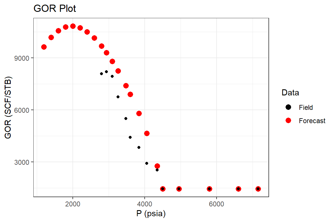
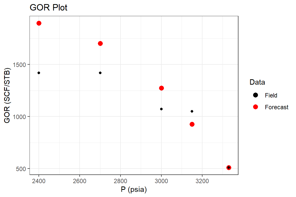
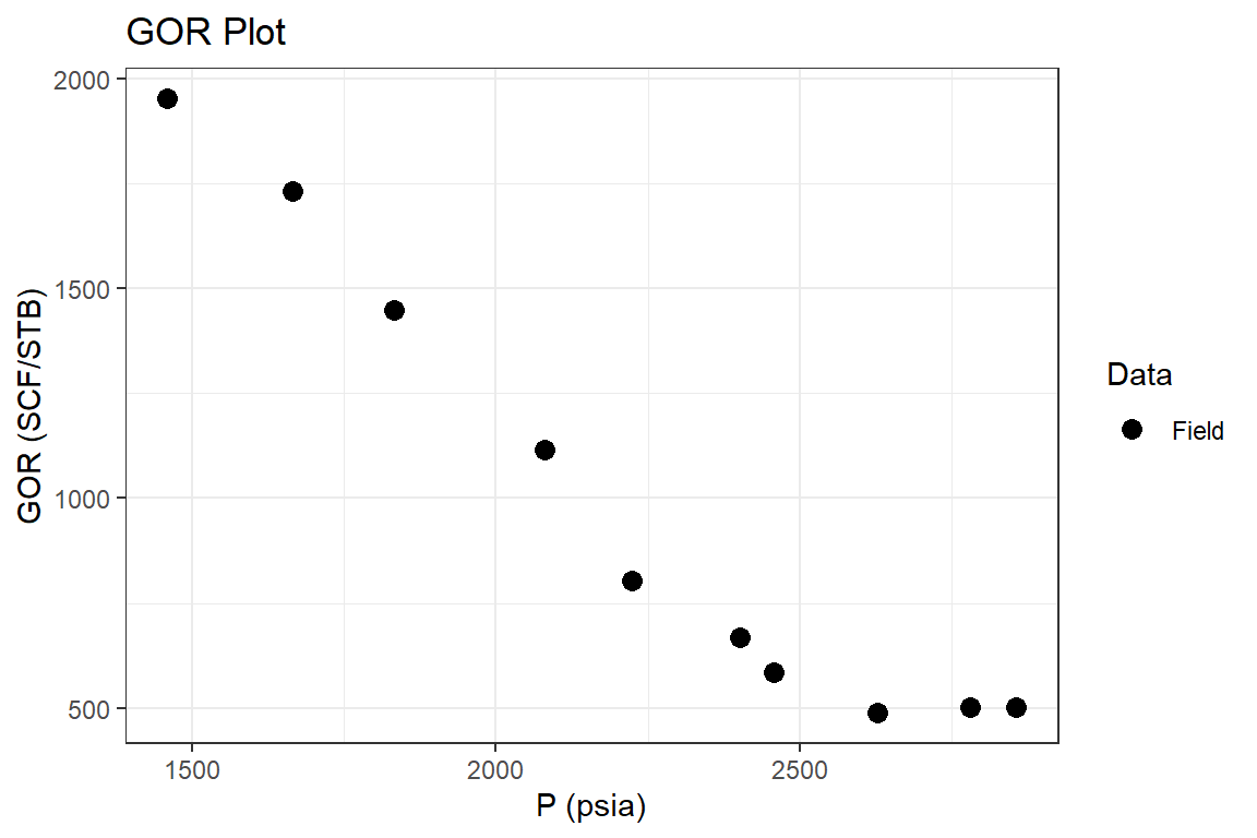
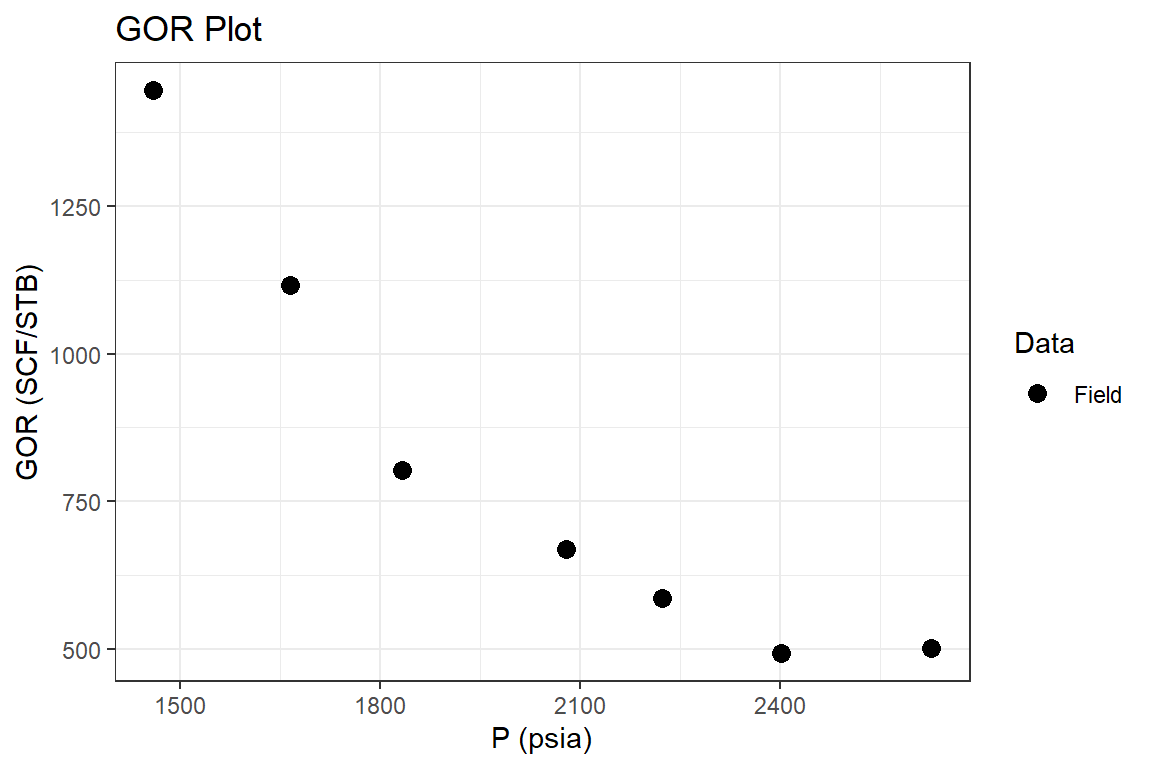
p2 <- forecast_results %>% ggplot(aes(`P (psia)`, `GOR (SCF/STB)`, color = "Forecast")) +
  geom_point(size = 3) +
  geom_point(data = mbal_results, aes(`P (psia)`, `GOR (SCF/STB)`, color = "Field"))+
  scale_color_manual(name="Data", values=c("Forecast" = "red", "Field" = "black")) +
  ggtitle("GOR Plot") +
  theme_bw()

p2
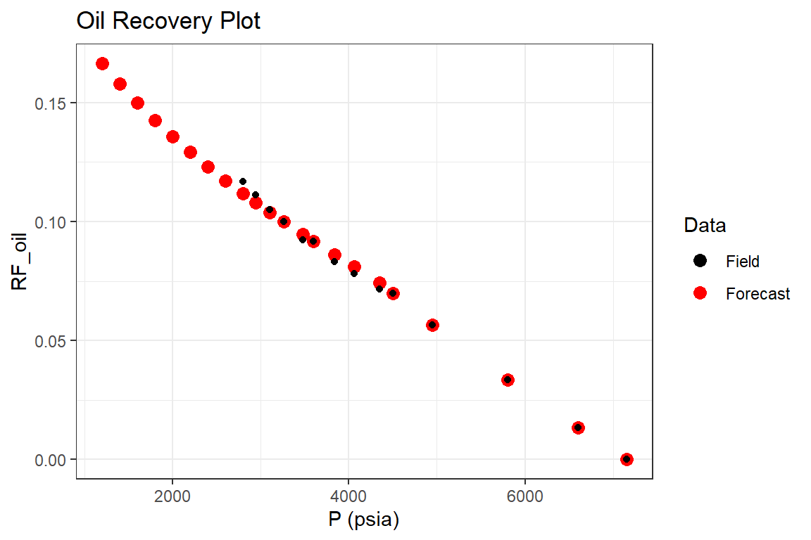
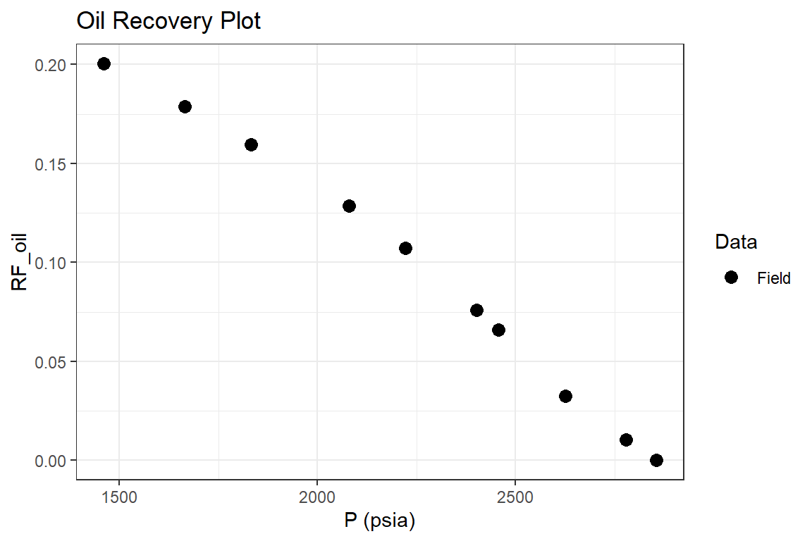
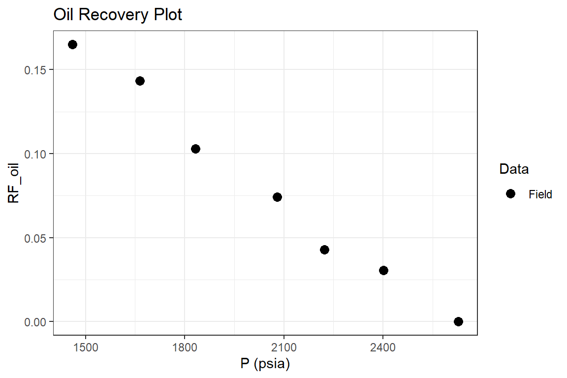
p3 <- forecast_results %>% ggplot(aes(`P (psia)`, `RF_oil`, color = "Forecast")) +
  geom_point(size = 3) +
  geom_point(data = mbal_results, aes(`P (psia)`, `RF_oil`, color = "Field"))+
  scale_color_manual(name="Data", values=c("Forecast" = "red", "Field" = "black")) +
  ggtitle("Oil Recovery Plot") +
  theme_bw()

p3
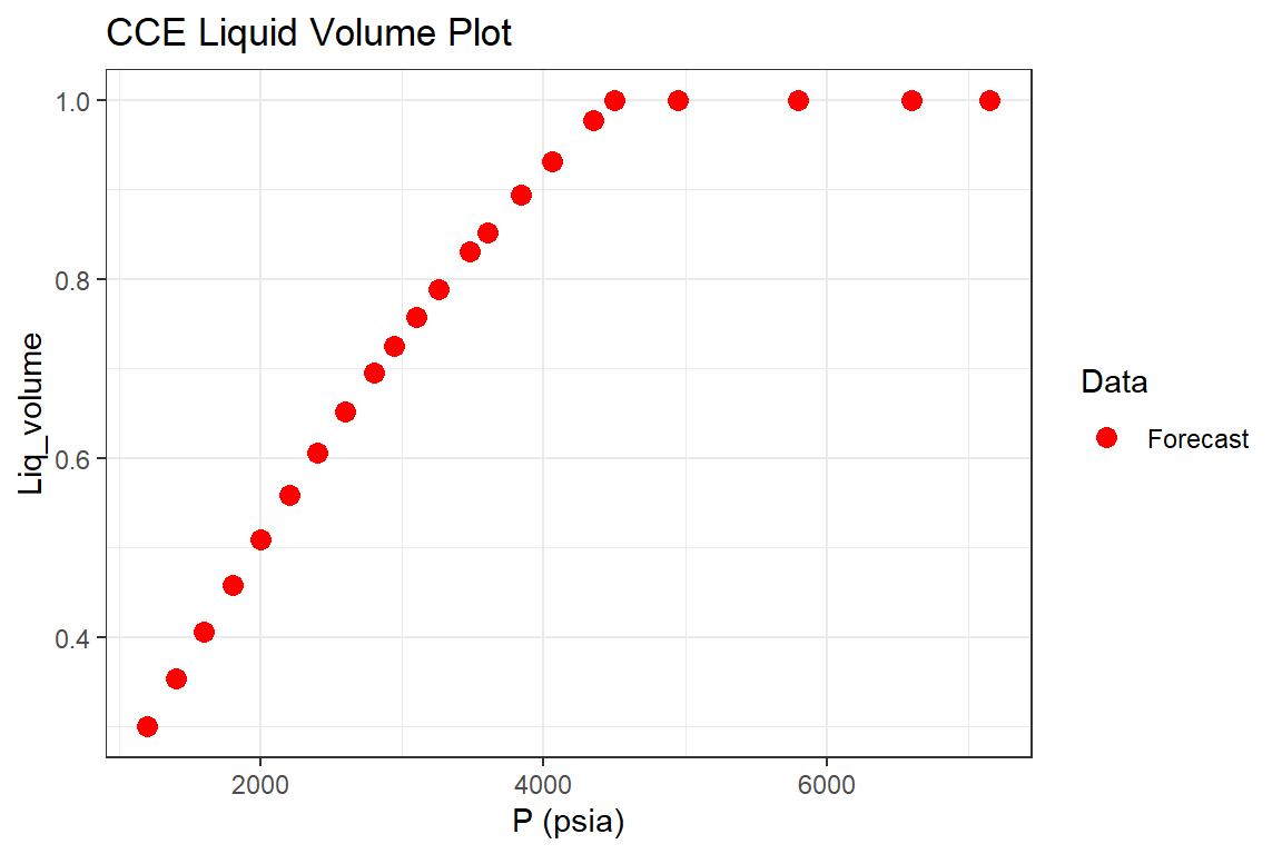
p4 <- forecast_results %>% ggplot(aes(`P (psia)`, `Liq_volume`, color = "Forecast")) +
  geom_point(size = 3) +
  scale_color_manual(name="Data", values=c("Forecast" = "red")) +
  ggtitle("CCE Liquid Volume Plot") +
  theme_bw()

p4
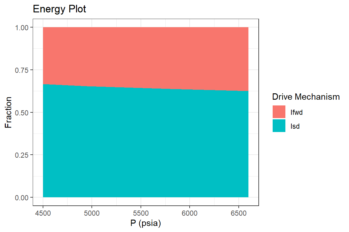
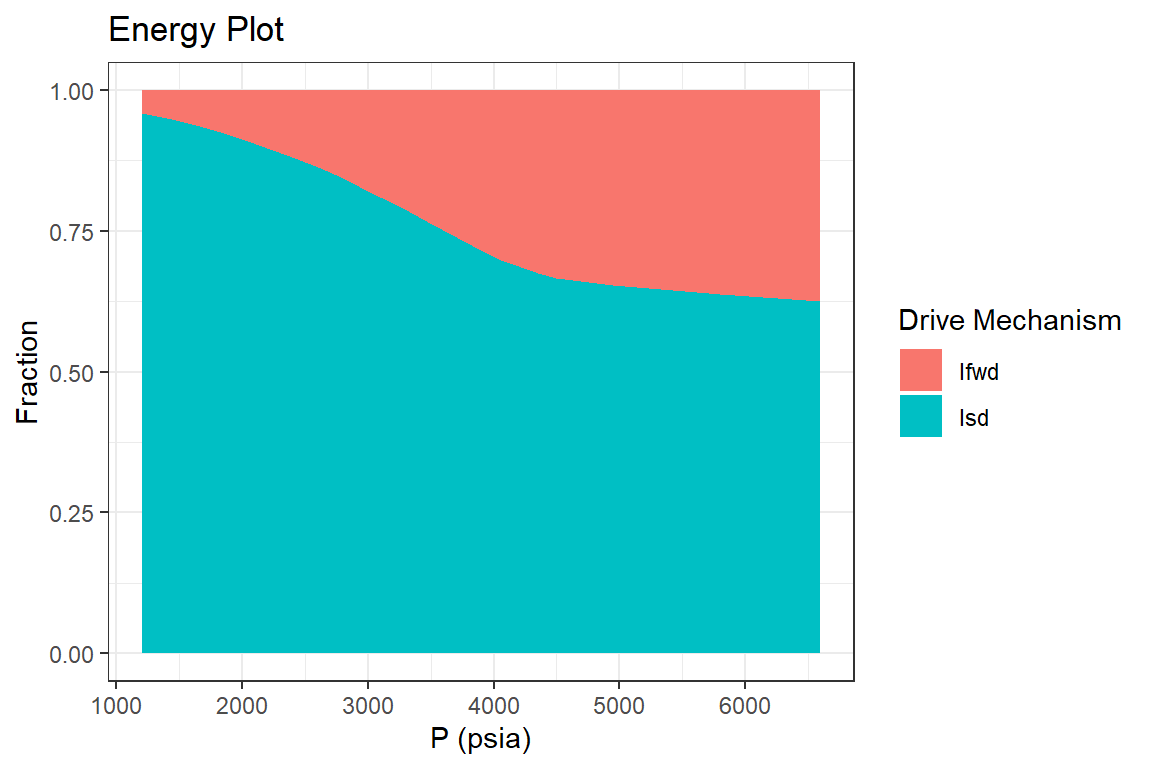
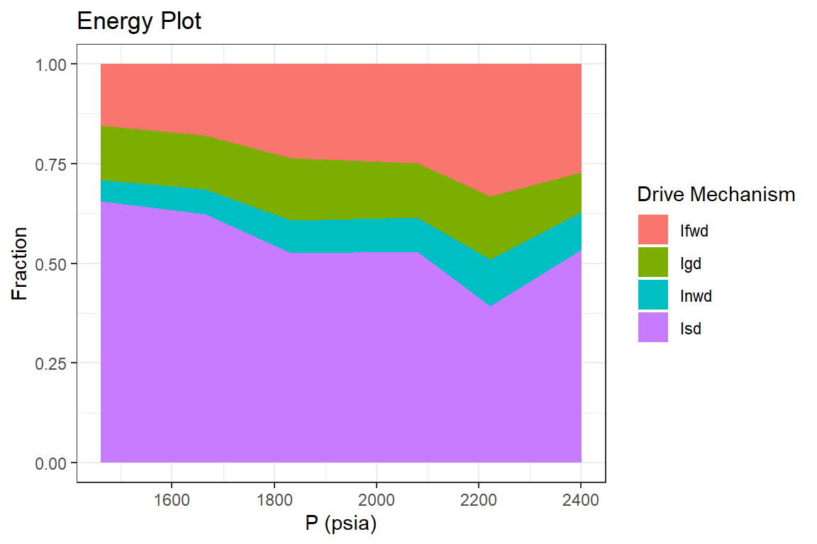
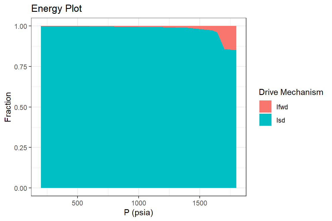
p5 <- forecast_results  %>%
  tidyr::pivot_longer(cols = c("Isd", "Ifwd"), names_to = "Drive Mechanism",
                      values_to = "Fraction", values_drop_na = TRUE) %>%
  ggplot(aes(`P (psia)`, Fraction, fill = `Drive Mechanism`)) +
  geom_area() +
  ggtitle("Energy Plot") +
  theme_bw()

p5
Example 3: Saturated Black Oil Reservoir with Gas Cap (Dake, 1983)
Part I: History Match
library(Rmbal)
library(Rrelperm)
library(pracma)
library(ggplot2)
library(dplyr)
library(magrittr)

p_pvt <- c(3330, 3150, 3000, 2850, 2700, 2550, 2400)

Bo <- c(1.2511, 1.2353, 1.2222, 1.2122, 1.2022, 1.1922, 1.1822)

Rs <- c(510, 477, 450, 425, 401, 375, 352)

Bg <- c(0.00087, 0.00092, 0.00096, 0.00101, 0.00107, 0.00113, 0.00120)

cw <- 2e-6

Bwi <- 1.0

Bw <- Bwi * exp(cw * (p_pvt[1] - p_pvt))

Rv <- rep(0, length(p_pvt))

muo <- rep(0.5, length(p_pvt))

muw <- rep(0.25, length(p_pvt))

mug <- rep(0.02, length(p_pvt))

pvt_table <- data.frame(p = p_pvt, Bo = Bo, Rs = Rs, Rv = Rv, Bg = Bg,
                               Bw = Bw, muo = muo, mug = mug, muw = muw)

p <- c(3330, 3150, 3000, 2850, 2700, 2550, 2400)

We <- rep(0, length.out = length(p))

Np <- c(0, 3.295, 5.903, 8.852, 11.503, 14.513, 17.730) * 1e6

Rp <- c(0, 1050, 1060, 1160, 1235, 1265, 1300)

Wp <- rep(0, length.out = length(p))

Wi <- rep(0, length.out = length(p))

Gi <- rep(0, length.out = length(p))

wf <- c(1, 1, 1, 0, 1, 0, 1)

mbal_optim_oil_lst <- mbal_optim_param_oil(input_unit = "Field", output_unit = "Field",
                                          unknown_param = "N_m", aquifer_model = NULL,
                                          phi = 0.2, swi = 0.2, Np = Np,
                                          Rp = Rp, Wp = Wp, Gi = Gi, Wi = Wi, We = We,
                                          pb = 3330, p = p, pvt = pvt_table, cf = 0,
                                          wf = wf, sorg = 0.2, sorw = 0)

time_lst <- mbal_time(c(0, 365, 730, 1095, 1460, 1825, 2190), "day")

# a number of plots will be automatically generated for quality check

optim_results <- mbal_optim_oil(mbal_optim_oil_lst, time_lst)
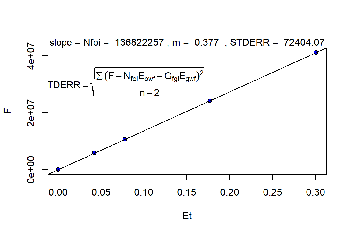
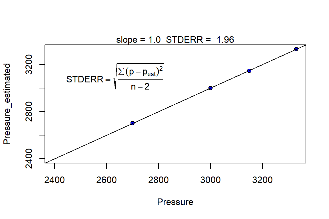
glimpse(optim_results)
#> List of 18
#>  $ input_unit : chr "Field"
#>  $ output_unit: chr "Field"
#>  $ N          : num 1.37e+08
#>  $ m          : num 0.377
#>  $ phi        : num 0.2
#>  $ swi        : num 0.2
#>  $ pb         : num 3330
#>  $ p          : num [1:7] 3330 3150 3000 2850 2700 2550 2400
#>  $ cf         : num [1:7] 0 0 0 0 0 0 0
#>  $ pvt        :'data.frame': 7 obs. of  9 variables:
#>   ..$ p  : num [1:7] 3330 3150 3000 2850 2700 2550 2400
#>   ..$ Bo : num [1:7] 1.25 1.24 1.22 1.21 1.2 ...
#>   ..$ Rs : num [1:7] 510 477 450 425 401 375 352
#>   ..$ Rv : num [1:7] 0 0 0 0 0 0 0
#>   ..$ Bg : num [1:7] 0.00087 0.00092 0.00096 0.00101 0.00107 0.00113 0.0012
#>   ..$ Bw : num [1:7] 1 1 1 1 1 ...
#>   ..$ muo: num [1:7] 0.5 0.5 0.5 0.5 0.5 0.5 0.5
#>   ..$ mug: num [1:7] 0.02 0.02 0.02 0.02 0.02 0.02 0.02
#>   ..$ muw: num [1:7] 0.25 0.25 0.25 0.25 0.25 0.25 0.25
#>  $ prod       :'data.frame': 7 obs. of  3 variables:
#>   ..$ Np: num [1:7] 0 3295000 5903000 8852000 11503000 ...
#>   ..$ Rp: num [1:7] 510 1050 1060 1160 1235 ...
#>   ..$ Wp: num [1:7] 0 0 0 0 0 0 0
#>  $ inj        :'data.frame': 7 obs. of  2 variables:
#>   ..$ Gi: num [1:7] 0 0 0 0 0 0 0
#>   ..$ Wi: num [1:7] 0 0 0 0 0 0 0
#>  $ We         : num [1:7] 0 0 0 0 0 0 0
#>  $ aquifer    :List of 3
#>   ..$ input_unit : chr "Field"
#>   ..$ output_unit: chr "Field"
#>   ..$ We         : num [1:7] 0 0 0 0 0 0 0
#>   ..- attr(*, "class")= chr [1:2] "NoA" "aquifer"
#>  $ wf         : num [1:7] 1 1 1 0 1 0 1
#>  $ sorw       : num 0
#>  $ sorg       : num 0.2
#>  $ p_est      : num [1:5] 3330 3147 2999 2702 NA
#>  - attr(*, "class")= chr [1:2] "gas_cap_oil" "mbal_oil"
Part II: Reservoir Performance
mbal_results <- mbal_perform_oil(optim_results, time_lst)

mbal_results
#>   P (psia) Eo (bbl/STB) Eg (bbl/SCF) Ew (bbl/STB) Ef (bbl/bbl) Eowf (bbl/STB)
#> 1     3330      0.00000      0.00000 0.0000000000            0     0.00000000
#> 2     3150      0.01456      0.00005 0.0003600648            0     0.01467262
#> 3     3000      0.02870      0.00009 0.0006602178            0     0.02890650
#> 4     2700      0.06773      0.00020 0.0012607941            0     0.06812434
#> 5     2400      0.12070      0.00033 0.0018617309            0     0.12128230
#>   Egwf (bbl/SCF) Et (bbl)  F (bbl) We       Igd       Isd Inwd        Ifwd Iawd
#> 1   0.000000e+00        0        0  0        NA        NA   NA          NA   NA
#> 2   5.007831e-05  5722033  5807306  0 0.6481408 0.3481511    0 0.003708064    0
#> 3   9.014360e-05 10641333 10671443  0 0.6273302 0.3690138    0 0.003656017    0
#> 4   2.002742e-04 24175999 24093954  0 0.6136140 0.3833129    0 0.003073100    0
#> 5   3.304049e-04 41101462 41130054  0 0.5955338 0.4017971    0 0.002669172    0
#>   Itot     RF_oil     RF_gas       SOo        SGo SWo       SOT       SGT SWT
#> 1   NA 0.00000000 0.00000000 0.8000000 0.00000000 0.2 0.5809809 0.2190191 0.2
#> 2    1 0.02372872 0.02368098 0.7833190 0.01668101 0.2 0.5598291 0.2401709 0.2
#> 3    1 0.04302183 0.04334418 0.7692774 0.03072257 0.2 0.5430738 0.2569262 0.2
#> 4    1 0.08435887 0.09902245 0.7520598 0.04794024 0.2 0.5113374 0.2886626 0.2
#> 5    1 0.12949410 0.16000344 0.7344800 0.06551996 0.2 0.4778455 0.3221545 0.2
#>   qo (STB/day) qg (SCF/day) qw (STB/day)        fg fw GOR (SCF/STB)    krg/kro
#> 1        0.000            0            0 0.0000000  0       510.000 0.00000000
#> 2     9027.397      9478767            0 0.2991047  0      1050.000 0.01706986
#> 3     7145.205      7664192            0 0.3403058  0      1072.634 0.01956239
#> 4     7671.233     10889075            0 0.4878215  0      1419.469 0.03625891
#> 5     8530.137     12113418            0 0.5404484  0      1420.073 0.04336619
Part III: Reservoir Forecast
# Step I: generating a set of pseudo relative permeability curves by minimizing
# the difference between field and theoretical 'fg' values
# 'swcrit' and 'sgcrit' values are estimated from the 'mbal_results' data frame

fun_fg <- function(x, swcrit, sgcrit, muo, mug, sg, fg, krg_kro) {
  Kr_table <- Rrelperm::kr2p_gl(SWCON = swcrit, SOIRG = x[1], SORG = x[1],
                                            SGCON = sgcrit, SGCRIT = sgcrit, KRGCL = x[2],
                                            KROGCG = x[3], NG = x[4], NOG = x[5], NP = 101)
  l <- length(fg)
  krg_est_sub <- vector(length = l)
  kro_est_sub <- vector(length = l)
  krg_est_sub <- approx(x = Kr_table[,1], y = Kr_table[,3], xout = sg, rule = 2)$y
  kro_est_sub <- approx(x = Kr_table[,1], y = Kr_table[,4], xout = sg, rule = 2)$y
  fg_est <- (krg_est_sub / mug) / (krg_est_sub / mug + kro_est_sub / muo)
  krg_kro_est <- krg_est_sub / kro_est_sub
  error <- (fg - fg_est) ^ 2 + (krg_kro - krg_kro_est) ^ 2
  return(error)
}

swcrit <- 0.2
sgcrit <- 0.00
p <- mbal_results$`P (psia)`
sg <- mbal_results$SGo  # gas saturation in the oil leg
fg <- mbal_results$fg   # in-situ gas fractional flow
krg_kro <- mbal_results$`krg/kro`
muo <- approx(x = pvt_table$p, y = pvt_table$muo, xout = p, rule = 2)$y
mug <- approx(x = pvt_table$p, y = pvt_table$mug, xout = p, rule = 2)$y

par <- c(0.1, 0.3, 1.0, 3, 3)
lower = c(0, 0.3, 1.0, 0.1, 0.1)
upper = c(1 - swcrit - sgcrit, 0.3, 1.0, 10.0, 10.0)
opt_results <- minpack.lm::nls.lm(par = par, fn = fun_fg, swcrit = swcrit, sgcrit = sgcrit,
                                  muo = muo, mug = mug, sg = sg, fg = fg, krg_kro = krg_kro,
                                  lower = lower, upper = upper)

opt_results
#> Nonlinear regression via the Levenberg-Marquardt algorithm
#> parameter estimates: 0, 0.3, 1, 0.926585263186008, 10
#> residual sum-of-squares: 0.000173
#> reason terminated: Relative error between `par' and the solution is at most `ptol'.

sol <- opt_results$par

sol
#> [1]  0.0000000  0.3000000  1.0000000  0.9265853 10.0000000

rel_perm <- as.data.frame(Rrelperm::kr2p_gl(SWCON = swcrit, SOIRG = sol[1], SORG = sol[1],
                                            SGCON = sgcrit, SGCRIT = sgcrit, KRGCL = sol[2],
                                            KROGCG = sol[3], NG = sol[4], NOG = sol[5],
                                            NP = 101))

colnames(rel_perm) <- c("Sg", "Sl", "Krg", "Krog")

krg_est <- approx(x = rel_perm[,1], y = rel_perm[,3], xout = sg, rule = 2)$y

kro_est <- approx(x = rel_perm[,1], y = rel_perm[,4], xout = sg, rule = 2)$y

fg_est <- (krg_est/ mug) / (krg_est / mug + kro_est / muo)

fg_df <- data.frame(Sg = sg)

fg_df$fg <- fg_est

p_fg <- fg_df %>% ggplot(aes(sg, fg, color = "Model")) +
  geom_point(size = 3) +
  geom_point(data = mbal_results, aes(SGo, fg, color = "Field"), size = 3)+
  xlim(c(0,1)) +
  ylim(c(0,1)) +
  scale_color_manual(name="Data", values=c("Model" = "red", "Field" = "black")) +
  ggtitle("Gas Frational Flow Plot") +
  theme_bw()

p_fg
p_forecast <- p_pvt

Gi_forecast <- c(Gi)

wf_forecast <- c(wf)

time_lst_forecast <- mbal_time(c(0, 365, 730, 1095, 1460, 1825, 2190), "day")

forecast_lst <- mbal_forecast_param_oil(input_unit = "Field", output_unit = "Field",
                                        N = 1.37e8, m = 0.377, phi = 0.2, swi = 0.2,
                                        Gi = Gi_forecast, pb = 3330, p = p_forecast, pvt = pvt_table,
                                        cf = 0, wf = wf_forecast, sorg = 0.2, rel_perm = rel_perm)

glimpse(forecast_lst)
#> List of 14
#>  $ input_unit : chr "Field"
#>  $ output_unit: chr "Field"
#>  $ N          : num 1.37e+08
#>  $ m          : num 0.377
#>  $ phi        : num 0.2
#>  $ swi        : num 0.2
#>  $ pb         : num 3330
#>  $ p          : num [1:7] 3330 3150 3000 2850 2700 2550 2400
#>  $ cf         : num [1:7] 0 0 0 0 0 0 0
#>  $ pvt        :'data.frame': 7 obs. of  9 variables:
#>   ..$ p  : num [1:7] 3330 3150 3000 2850 2700 2550 2400
#>   ..$ Bo : num [1:7] 1.25 1.24 1.22 1.21 1.2 ...
#>   ..$ Rs : num [1:7] 510 477 450 425 401 375 352
#>   ..$ Rv : num [1:7] 0 0 0 0 0 0 0
#>   ..$ Bg : num [1:7] 0.00087 0.00092 0.00096 0.00101 0.00107 0.00113 0.0012
#>   ..$ Bw : num [1:7] 1 1 1 1 1 ...
#>   ..$ muo: num [1:7] 0.5 0.5 0.5 0.5 0.5 0.5 0.5
#>   ..$ mug: num [1:7] 0.02 0.02 0.02 0.02 0.02 0.02 0.02
#>   ..$ muw: num [1:7] 0.25 0.25 0.25 0.25 0.25 0.25 0.25
#>  $ inj        :'data.frame': 7 obs. of  1 variable:
#>   ..$ Gi: num [1:7] 0 0 0 0 0 0 0
#>  $ wf         : num [1:7] 1 1 1 0 1 0 1
#>  $ sorg       : num 0.2
#>  $ rel_perm   :'data.frame': 101 obs. of  4 variables:
#>   ..$ Sg  : num [1:101] 0 0.01 0.02 0.03 0.04 0.05 0.06 0.07 0.08 0.09 ...
#>   ..$ Sl  : num [1:101] 1 0.99 0.98 0.97 0.96 0.95 0.94 0.93 0.92 0.91 ...
#>   ..$ Krg : num [1:101] 0 0.00517 0.00983 0.01432 0.01869 ...
#>   ..$ Krog: num [1:101] 1 0.882 0.776 0.682 0.599 ...
#>  - attr(*, "class")= chr [1:2] "gas_cap_forecast_oil" "forecast_oil"


forecast_results <- mbal_forecast_oil(forecast_lst, time_lst_forecast)

forecast_results
#>   P (psia)       SOo        SGo SWo       SOT       SGT SWT GOR (SCF/STB)
#> 1     3330 0.8000000 0.00000000 0.2 0.5809731 0.2190269 0.2      510.0000
#> 2     3150 0.7790250 0.02097502 0.2 0.5571724 0.2428276 0.2      926.3694
#> 3     3000 0.7648711 0.03512886 0.2 0.5404104 0.2595896 0.2     1274.2193
#> 4     2700 0.7481436 0.05185644 0.2 0.5091204 0.2908796 0.2     1704.3453
#> 5     2400 0.7379930 0.06200705 0.2 0.4796626 0.3203374 0.2     1898.0197
#>       RF_oil     RF_gas Liq_volume       Igd       Isd Inwd        Ifwd Iawd
#> 1 0.00000000 0.00000000  1.0000000        NA        NA   NA          NA   NA
#> 2 0.02870061 0.01959081  0.9760125 0.6481519 0.3481401    0 0.003707997    0
#> 3 0.04782355 0.03958891  0.9549930 0.6273415 0.3690025    0 0.003655953    0
#> 4 0.08803163 0.09650242  0.9115656 0.6136256 0.3833014    0 0.003073049    0
#> 5 0.12626274 0.16195092  0.8617874 0.5955455 0.4017854    0 0.002669130    0
#>   Itot
#> 1   NA
#> 2    1
#> 3    1
#> 4    1
#> 5    1

p1 <- forecast_results %>% ggplot(aes(`P (psia)`, SOo, color = "Forecast")) +
  geom_point(size = 3) +
  geom_point(data = mbal_results, aes(`P (psia)`, SOo, color = "Field"))+
  scale_color_manual(name="Data", values=c("Forecast" = "red", "Field" = "black")) +
  ggtitle("Oil Saturation Plot") +
  theme_bw()

p1
p2 <- forecast_results %>% ggplot(aes(`P (psia)`, `GOR (SCF/STB)`, color = "Forecast")) +
  geom_point(size = 3) +
  geom_point(data = mbal_results, aes(`P (psia)`, `GOR (SCF/STB)`, color = "Field"))+
  scale_color_manual(name="Data", values=c("Forecast" = "red", "Field" = "black")) +
  ggtitle("GOR Plot") +
  theme_bw()

p2
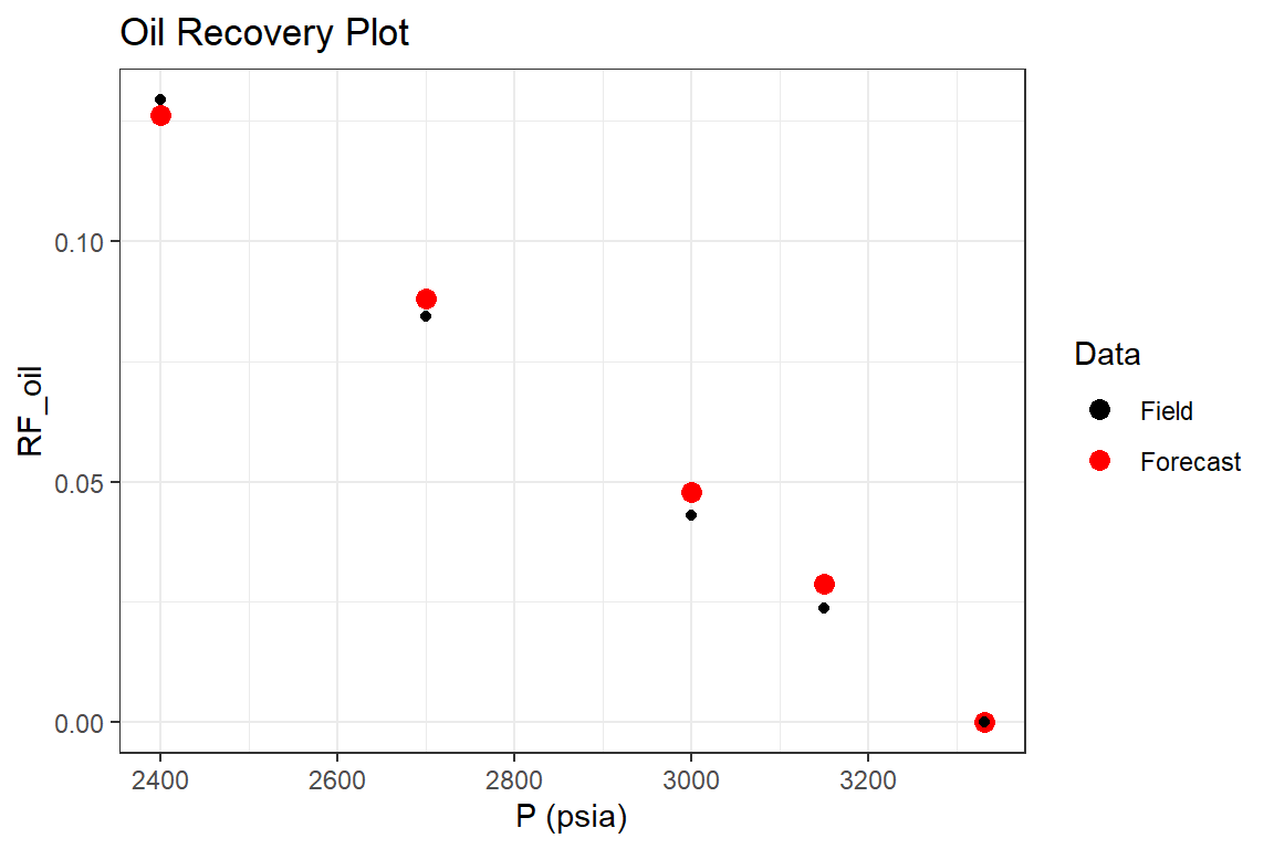
p3 <- forecast_results %>% ggplot(aes(`P (psia)`, `RF_oil`, color = "Forecast")) +
  geom_point(size = 3) +
  geom_point(data = mbal_results, aes(`P (psia)`, `RF_oil`, color = "Field"))+
  scale_color_manual(name="Data", values=c("Forecast" = "red", "Field" = "black")) +
  ggtitle("Oil Recovery Plot") +
  theme_bw()

p3
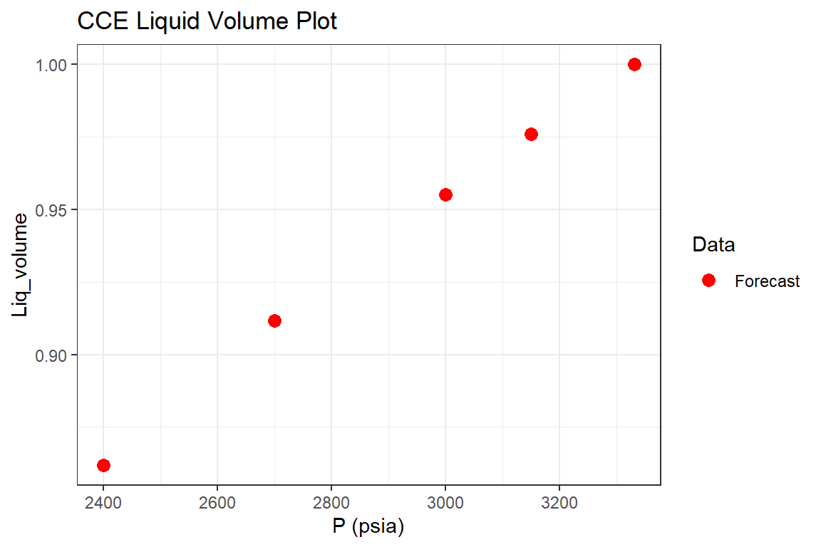
p4 <- forecast_results %>% ggplot(aes(`P (psia)`, `Liq_volume`, color = "Forecast")) +
  geom_point(size = 3) +
  scale_color_manual(name="Data", values=c("Forecast" = "red")) +
  ggtitle("CCE Liquid Volume Plot") +
  theme_bw()

p4
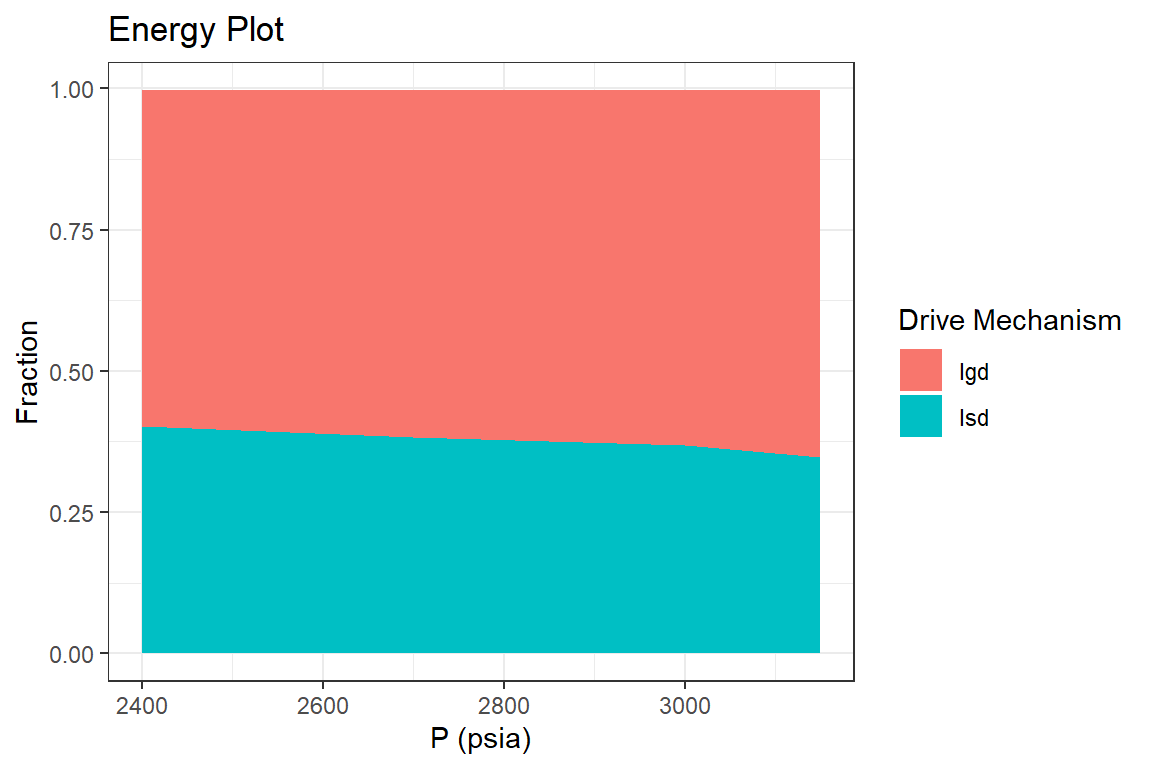
p5 <- forecast_results  %>%
  tidyr::pivot_longer(cols = c("Igd", "Isd"), names_to = "Drive Mechanism",
                      values_to = "Fraction", values_drop_na = TRUE) %>%
  ggplot(aes(`P (psia)`, Fraction, fill = `Drive Mechanism`)) +
  geom_area() +
  ggtitle("Energy Plot") +
  theme_bw()

p5
Example 4: Water-Drive Saturated Black Oil Reservoir (Dake, 1983)
Part I: History Match
library(Rmbal)
library(Rrelperm)
library(pracma)
library(ggplot2)
library(dplyr)
library(magrittr)

p_pvt <- c(2740, 2500, 2290, 2109, 1949, 1818, 1702, 1608, 1535, 1480, 1440)

Bo <- c(1.404, 1.374, 1.349, 1.329, 1.316, 1.303, 1.294, 1.287, 1.280, 1.276, 1.273)

Rs <- c(650, 592, 545, 507, 471, 442, 418, 398, 383, 371, 364)

Bg <- c(0.00093, 0.00098, 0.00107, 0.00117, 0.00128, 0.00139, 0.00150, 0.00160,
        0.00170, 0.00176, 0.00182)

cw <- 3e-6

Bwi <- 1.0

Bw <- Bwi * exp(cw * (p_pvt[1] - p_pvt))

Rv <- rep(0, length(p_pvt))

muo <- rep(0.5, length(p_pvt))

muw <- rep(0.55, length(p_pvt))

mug <- rep(0.02, length(p_pvt))

pvt_table <- data.frame(p = p_pvt, Bo = Bo, Rs = Rs, Rv = Rv, Bg = Bg,
                               Bw = Bw, muo = muo, mug = mug, muw = muw)

p <- c(2740, 2500, 2290, 2109, 1949, 1818, 1702, 1608, 1535, 1480, 1440)

We <- rep(0, length.out = length(p))

Np <- c(0, 7.88, 18.42, 29.15, 40.69, 50.14, 58.42, 65.39, 70.74, 74.54, 77.43) * 1e6

Rp <- c(0, 760, 845, 920, 975, 1025, 1065, 1095, 1120, 1145, 1160)

Wp <- rep(0, length.out = length(p))

Wi <- rep(0, length.out = length(p))

Gi <- rep(0, length.out = length(p))

wf <- rep(1, length.out = length(p))

mbal_optim_oil_lst <- mbal_optim_param_oil(input_unit = "Field", output_unit = "Field",
                                           unknown_param = "We",
                                           aquifer_model = "pss_rad_edge", N = 312e6,
                                           m = 0, phi = 0.25, swi = 0.25, Np = Np, Rp = Rp,
                                           Wp = Wp, Gi = Gi, Wi = Wi, We = NULL, pb = 2740,
                                           p = p, pvt = pvt_table, cf = 4e-6,
                                           phi_a = 0.25, perm_h_a = 200, h_a = 100,
                                           r_a = 5 * 9200, r_R = 9200, tetha = 140,
                                           muw_a = 0.55, cw_a = 3e-6, cf_a = 4e-6,
                                           wf = wf, sorw = 0.2, sorg = 0,
                                           mult_len = c(1,1), lower = c(-Inf, 1),
                                           upper = c(Inf, 1),
                                           control = list(maxiter = 100), )

time_lst <- mbal_time(0:10, "year")

# a number of plots will be automatically generated for quality check

optim_results <- mbal_optim_oil(mbal_optim_oil_lst, time_lst)
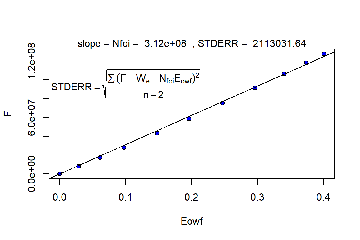
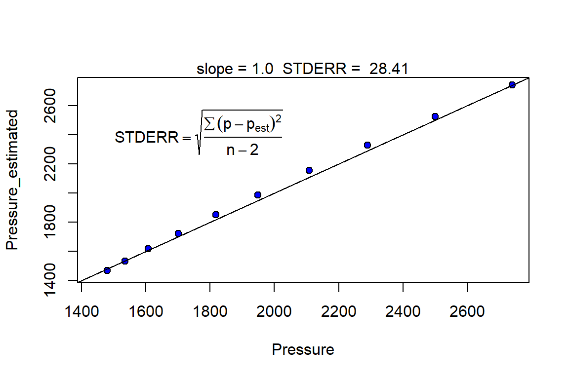
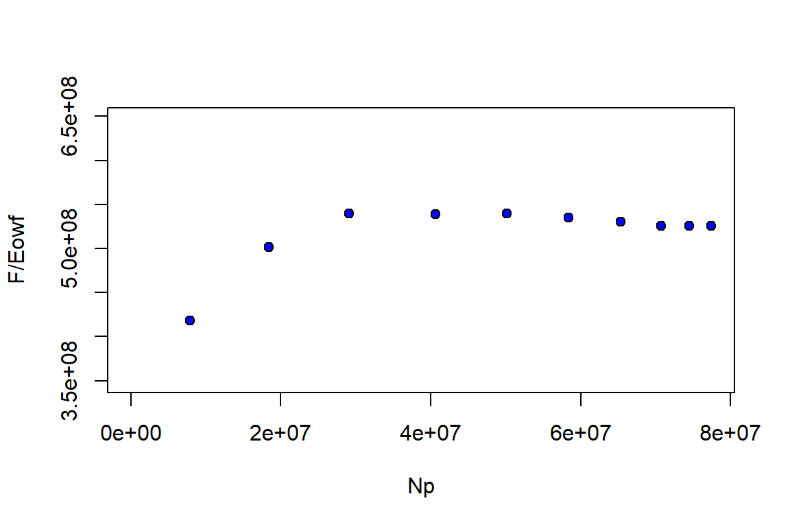
glimpse(optim_results)
#> List of 18
#>  $ input_unit : chr "Field"
#>  $ output_unit: chr "Field"
#>  $ N          : num 3.12e+08
#>  $ m          : num 0
#>  $ phi        : num 0.25
#>  $ swi        : num 0.25
#>  $ pb         : num 2740
#>  $ p          : num [1:11] 2740 2500 2290 2109 1949 ...
#>  $ cf         : num [1:11] 4e-06 4e-06 4e-06 4e-06 4e-06 4e-06 4e-06 4e-06 4e-06 4e-06 ...
#>  $ pvt        :'data.frame': 11 obs. of  9 variables:
#>   ..$ p  : num [1:11] 2740 2500 2290 2109 1949 ...
#>   ..$ Bo : num [1:11] 1.4 1.37 1.35 1.33 1.32 ...
#>   ..$ Rs : num [1:11] 650 592 545 507 471 442 418 398 383 371 ...
#>   ..$ Rv : num [1:11] 0 0 0 0 0 0 0 0 0 0 ...
#>   ..$ Bg : num [1:11] 0.00093 0.00098 0.00107 0.00117 0.00128 0.00139 0.0015 0.0016 0.0017 0.00176 ...
#>   ..$ Bw : num [1:11] 1 1 1 1 1 ...
#>   ..$ muo: num [1:11] 0.5 0.5 0.5 0.5 0.5 0.5 0.5 0.5 0.5 0.5 ...
#>   ..$ mug: num [1:11] 0.02 0.02 0.02 0.02 0.02 0.02 0.02 0.02 0.02 0.02 ...
#>   ..$ muw: num [1:11] 0.55 0.55 0.55 0.55 0.55 0.55 0.55 0.55 0.55 0.55 ...
#>  $ prod       :'data.frame': 11 obs. of  3 variables:
#>   ..$ Np: num [1:11] 0 7880000 18420000 29150000 40690000 ...
#>   ..$ Rp: num [1:11] 650 760 845 920 975 ...
#>   ..$ Wp: num [1:11] 0 0 0 0 0 0 0 0 0 0 ...
#>  $ inj        :'data.frame': 11 obs. of  2 variables:
#>   ..$ Gi: num [1:11] 0 0 0 0 0 0 0 0 0 0 ...
#>   ..$ Wi: num [1:11] 0 0 0 0 0 0 0 0 0 0 ...
#>  $ We         : NULL
#>  $ aquifer    :List of 14
#>   ..$ input_unit : chr "Field"
#>   ..$ output_unit: chr "Field"
#>   ..$ model      : chr "pss_rad_edge"
#>   ..$ phi        : num 0.25
#>   ..$ perm_h     : num 200
#>   ..$ h_a        : num 100
#>   ..$ r_a        : num 43487
#>   ..$ r_R        : num 9200
#>   ..$ tetha      : num 140
#>   ..$ mu_water   : num 0.55
#>   ..$ c_water    : num 3e-06
#>   ..$ c_rock     : num 4e-06
#>   ..$ pressure   : num [1:11] 2740 2500 2290 2109 1949 ...
#>   ..$ mult_len   : num [1:2] 1 1
#>   ..- attr(*, "class")= chr [1:2] "pss_rad_edge" "aquifer"
#>  $ wf         : num [1:11] 1 1 1 1 1 1 1 1 1 1 ...
#>  $ sorw       : num 0.2
#>  $ sorg       : num 0
#>  $ p_est      : num [1:11] 2740 2523 2330 2156 1986 ...
#>  - attr(*, "class")= chr [1:2] "water_drive_oil" "mbal_oil"
Part II: Reservoir Performance
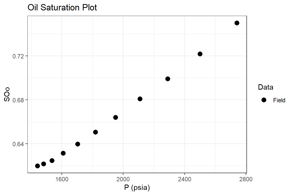
mbal_results <- mbal_perform_oil(optim_results, time_lst)

mbal_results
#>    P (psia) Eo (bbl/STB) Eg (bbl/SCF) Ew (bbl/STB) Ef (bbl/bbl) Eowf (bbl/STB)
#> 1      2740      0.00000      0.00000 0.0000000000     0.000000     0.00000000
#> 2      2500      0.02684      0.00005 0.0007202593     0.000960     0.02897420
#> 3      2290      0.05735      0.00014 0.0013509117     0.001800     0.06135183
#> 4      2109      0.09231      0.00024 0.0018947929     0.002524     0.09792169
#> 5      1949      0.14112      0.00035 0.0023758178     0.003164     0.14815489
#> 6      1818      0.18812      0.00046 0.0027698289     0.003688     0.19632022
#> 7      1702      0.23800      0.00057 0.0031188535     0.004152     0.24723217
#> 8      1608      0.28620      0.00067 0.0034017729     0.004528     0.29626845
#> 9      1535      0.32990      0.00077 0.0036215420     0.004820     0.34061792
#> 10     1480      0.36304      0.00083 0.0037871532     0.005040     0.37424727
#> 11     1440      0.38952      0.00089 0.0039076149     0.005200     0.40108316
#>    Egwf (bbl/SCF)  Et (bbl)   F (bbl)       We Igd       Isd      Inwd
#> 1    0.000000e+00         0         0        0  NA        NA        NA
#> 2    5.141368e-05  13033980  12124483  3994030   0 0.6424806 0.3064321
#> 3    1.426508e-04  32685981  30761400 13544211   0 0.5474273 0.4143737
#> 4    2.437171e-04  55531705  52825922 24980137   0 0.5186356 0.4498356
#> 5    3.546599e-04  82781560  79797973 36557234   0 0.5318750 0.4416108
#> 6    4.654318e-04 108627009 105964372 47375101   0 0.5403209 0.4361264
#> 7    5.761153e-04 134205317 132292090 57068881   0 0.5533015 0.4252356
#> 8    6.766693e-04 158002511 157079858 65566756   0 0.5651454 0.4149729
#> 9    7.770995e-04 179004602 179177346 72731810   0 0.5750064 0.4063125
#> 10   8.374236e-04 195325095 196654410 78559947   0 0.5798972 0.4022010
#> 11   8.976594e-04 208286850 210742780 83148903   0 0.5834753 0.3992038
#>          Ifwd Iawd Itot     RF_oil     RF_gas       SOo        SGo  SWo
#> 1          NA   NA   NA 0.00000000 0.00000000 0.7500000 0.00000000 0.25
#> 2  0.05108730    0    1 0.02715098 0.03174576 0.7219261 0.02807391 0.25
#> 3  0.03819894    0    1 0.06273219 0.08155185 0.6991197 0.05088028 0.25
#> 4  0.03152879    0    1 0.09821502 0.13901202 0.6810118 0.06898825 0.25
#> 5  0.02651419    0    1 0.13529285 0.20293927 0.6641284 0.08587157 0.25
#> 6  0.02355277    0    1 0.16474327 0.25978747 0.6506495 0.09935045 0.25
#> 7  0.02146291    0    1 0.18995153 0.31122828 0.6399722 0.11002776 0.25
#> 8  0.01988168    0    1 0.21081438 0.35514115 0.6314801 0.11851989 0.25
#> 9  0.01868104    0    1 0.22651218 0.39029791 0.6249439 0.12505610 0.25
#> 10 0.01790178    0    1 0.23729531 0.41800481 0.6219729 0.12802707 0.25
#> 11 0.01732086    0    1 0.24528095 0.43773215 0.6199618 0.13003822 0.25
#>          SOT        SGT       SWT qo (STB/day) qg (SCF/day) qw (STB/day)
#> 1  0.7500000 0.00000000 0.2500000        0.000            0            0
#> 2  0.7154368 0.02772486 0.2568383    21589.041     16407671            0
#> 3  0.6780754 0.04873502 0.2731896    28876.712     26235890            0
#> 4  0.6436070 0.06362353 0.2927695    29397.260     30830411            0
#> 5  0.6113097 0.07609920 0.3125911    31616.438     35218493            0
#> 6  0.5841887 0.08469846 0.3311129    25890.411     32111644            0
#> 7  0.5618092 0.09048084 0.3477100    22684.932     29654247            0
#> 8  0.5434115 0.09432900 0.3622595    19095.890     25711644            0
#> 9  0.5287311 0.09674178 0.3745271    14657.534     20895205            0
#> 10 0.5187770 0.09671730 0.3845057    10410.959     16765753            0
#> 11 0.5112584 0.09637897 0.3923627     7917.808     12247945            0
#>           fg fw GOR (SCF/STB)     krg/kro
#> 1  0.0000000  0      650.0000 0.000000000
#> 2  0.1070036  0      760.0000 0.004793013
#> 3  0.2402547  0      908.5484 0.011534374
#> 4  0.3482651  0     1048.7512 0.019077468
#> 5  0.4164981  0     1113.9298 0.025013683
#> 6  0.4961705  0     1240.2910 0.034063684
#> 7  0.5453001  0     1307.2222 0.041231324
#> 8  0.5811543  0     1346.4491 0.047164522
#> 9  0.6195034  0     1425.5607 0.055386040
#> 10 0.6686145  0     1610.3947 0.068380399
#> 11 0.6609354  0     1546.8858 0.067646573

p1 <- mbal_results %>% ggplot(aes(`P (psia)`, SOo, color = "Field")) +
  geom_point(size = 3) +
  scale_color_manual(name="Data", values=c("Field" = "black")) +
  ggtitle("Oil Saturation Plot") +
  theme_bw()

p1
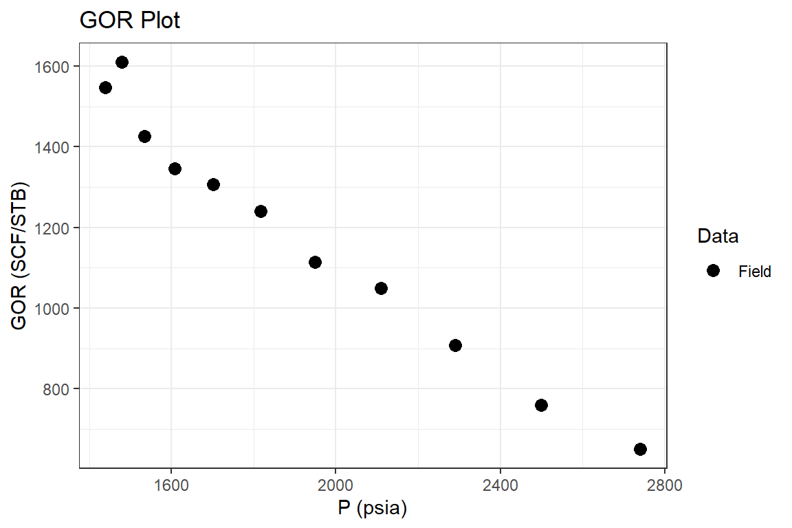
p2 <- mbal_results %>% ggplot(aes(`P (psia)`, `GOR (SCF/STB)`, color = "Field")) +
  geom_point(size = 3) +
  scale_color_manual(name="Data", values = c("Field" = "black")) +
  ggtitle("GOR Plot") +
  theme_bw()

p2
p3 <- mbal_results %>% ggplot(aes(`P (psia)`, `RF_oil`, color = "Field")) +
  geom_point(size = 3) +
  scale_color_manual(name="Data", values=c("Field" = "black")) +
  ggtitle("Oil Recovery Plot") +
  theme_bw()

p3
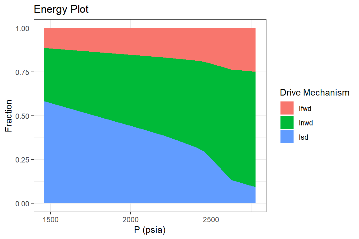
p4 <- mbal_results  %>%
  tidyr::pivot_longer(cols = c("Isd", "Inwd", "Ifwd"), names_to = "Drive Mechanism",
                      values_to = "Fraction", values_drop_na = TRUE) %>%
  ggplot(aes(`P (psia)`, Fraction, fill = `Drive Mechanism`)) +
  geom_area() +
  ggtitle("Energy Plot") +
  theme_bw()

p4
Example 5: Water-Drive Saturated Black Oil Reservoir (Pletcher, 2002)
Part I: History Match
library(Rmbal)
library(Rrelperm)
library(pracma)
library(ggplot2)
library(dplyr)
library(magrittr)

p_pvt <- c(2855,    2779,   2627,   2457,   2402,   2223,   2080,   1833,   1665,   1460)  # psia

Bo <- c(1.2665, 1.2677, 1.2681, 1.2554, 1.2512, 1.2383, 1.2278, 1.2074, 1.1949,
        1.1802)  # RB/STB

Rs <- c(0.501, 0.501,   0.4973, 0.4671, 0.4574, 0.4269, 0.4024, 0.3579, 0.3277,
        0.2908) * 1000  #SCF/STB

Bg <- c(0.9201, 0.9637, 1.0502, 1.0977, 1.1146, 1.201, 1.2825, 1.4584, 1.6112,
        1.8526) / 1000  # RB/SCF

Bw <- c(1.0222, 1.0224, 1.0228, 1.0232, 1.0233, 1.0237, 1.024,  1.0246, 1.025,
        1.0254)  # RB/STB

Rv <- rep(0, length(p_pvt))

muo <- rep(0.5, length(p_pvt))

muw <- rep(0.55, length(p_pvt))

mug <- rep(0.02, length(p_pvt))

pvt_table <- data.frame(p = p_pvt, Bo = Bo, Rs = Rs, Rv = Rv, Bg = Bg,
                               Bw = Bw, muo = muo, mug = mug, muw = muw)

p <- c(2855,    2779,   2627,   2457,   2402,   2223,   2080,   1833,   1665,   1460)  # psia

Np <- c(0,  192821, 633942, 1314880,    1524400,    2152960,    2572000,    3200560,
        3584680,    4003720)  # STB

Rp <- c(0,  501,    492.2595442,    540.4827817,    558.2091315,    629.7005054,
        708.8841369,    853.8693229,    947.8502963,    1053.050663)  # SCF/STB

Wp <- rep(0, length.out = length(p))

Wi <- rep(0, length.out = length(p))

Gi <- rep(0, length.out = length(p))

wf <- rep(1, length.out = length(p))

mbal_optim_oil_lst <- mbal_optim_param_oil(input_unit = "Field", output_unit = "Field",
                                           unknown_param = "We",
                                           aquifer_model = "pot", N = 20e6,
                                           m = 0, phi = 0.28, swi = 0.208, Np = Np,
                                           Rp = Rp, Wp = Wp, Gi = Gi, Wi = Wi,
                                           We = NULL, pb = 2648, p = p, pvt = pvt_table,
                                           cf = 26e-6, phi_a = 0.28, h_a = 200, r_a = 1000,
                                           r_R = 300, tetha = 360, cw_a = 2.28e-6,
                                           cf_a = 26e-6, mult_len = 3, wf = wf,
                                           sorw = 0.0, sorg = 0)

time_lst <- mbal_time(c(0,305, 700, 1285, 1465, 2005, 2365, 2905, 3235, 3595), "day")

# a number of plots will be automatically generated for quality check

optim_results <- mbal_optim_oil(mbal_optim_oil_lst, time_lst)
glimpse(optim_results)
#> List of 18
#>  $ input_unit : chr "Field"
#>  $ output_unit: chr "Field"
#>  $ N          : num 2e+07
#>  $ m          : num 0
#>  $ phi        : num 0.28
#>  $ swi        : num 0.208
#>  $ pb         : num 2648
#>  $ p          : num [1:10] 2855 2779 2627 2457 2402 ...
#>  $ cf         : num [1:10] 2.6e-05 2.6e-05 2.6e-05 2.6e-05 2.6e-05 2.6e-05 2.6e-05 2.6e-05 2.6e-05 2.6e-05
#>  $ pvt        :'data.frame': 10 obs. of  9 variables:
#>   ..$ p  : num [1:10] 2855 2779 2627 2457 2402 ...
#>   ..$ Bo : num [1:10] 1.27 1.27 1.27 1.26 1.25 ...
#>   ..$ Rs : num [1:10] 501 501 497 467 457 ...
#>   ..$ Rv : num [1:10] 0 0 0 0 0 0 0 0 0 0
#>   ..$ Bg : num [1:10] 0.00092 0.000964 0.00105 0.001098 0.001115 ...
#>   ..$ Bw : num [1:10] 1.02 1.02 1.02 1.02 1.02 ...
#>   ..$ muo: num [1:10] 0.5 0.5 0.5 0.5 0.5 0.5 0.5 0.5 0.5 0.5
#>   ..$ mug: num [1:10] 0.02 0.02 0.02 0.02 0.02 0.02 0.02 0.02 0.02 0.02
#>   ..$ muw: num [1:10] 0.55 0.55 0.55 0.55 0.55 0.55 0.55 0.55 0.55 0.55
#>  $ prod       :'data.frame': 10 obs. of  3 variables:
#>   ..$ Np: num [1:10] 0 192821 633942 1314880 1524400 ...
#>   ..$ Rp: num [1:10] 501 501 492 540 558 ...
#>   ..$ Wp: num [1:10] 0 0 0 0 0 0 0 0 0 0
#>  $ inj        :'data.frame': 10 obs. of  2 variables:
#>   ..$ Gi: num [1:10] 0 0 0 0 0 0 0 0 0 0
#>   ..$ Wi: num [1:10] 0 0 0 0 0 0 0 0 0 0
#>  $ We         : NULL
#>  $ aquifer    :List of 12
#>   ..$ input_unit : chr "Field"
#>   ..$ output_unit: chr "Field"
#>   ..$ model      : chr "pot"
#>   ..$ phi        : num 0.28
#>   ..$ h_a        : num 200
#>   ..$ r_a        : num 1625
#>   ..$ r_R        : num 300
#>   ..$ tetha      : num 360
#>   ..$ c_water    : num 2.28e-06
#>   ..$ c_rock     : num 2.6e-05
#>   ..$ pressure   : num [1:10] 2855 2779 2627 2457 2402 ...
#>   ..$ mult_len   : num 1
#>   ..- attr(*, "class")= chr [1:2] "pot" "aquifer"
#>  $ wf         : num [1:10] 1 1 1 1 1 1 1 1 1 1
#>  $ sorw       : num 0
#>  $ sorg       : num 0
#>  $ p_est      : num [1:10] 2855 2793 2639 2458 2400 ...
#>  - attr(*, "class")= chr [1:2] "water_drive_oil" "mbal_oil"
Part II: Reservoir Performance
mbal_results <- mbal_perform_oil(optim_results, time_lst)

mbal_results
#>    P (psia) Eo (bbl/STB) Eg (bbl/SCF) Ew (bbl/STB) Ef (bbl/bbl) Eowf (bbl/STB)
#> 1      2855   0.00000000    0.0000000       0.0000     0.000000    0.000000000
#> 2      2779   0.00120000    0.0000436       0.0002     0.001976    0.004424932
#> 3      2627   0.00548574    0.0001301       0.0006     0.005928    0.015160536
#> 4      2457   0.02611203    0.0001776       0.0010     0.010348    0.042985076
#> 5      2402   0.03329656    0.0001945       0.0011     0.011778    0.052488882
#> 6      2223   0.06079410    0.0002809       0.0015     0.016432    0.087558865
#> 7      2080   0.08775450    0.0003624       0.0018     0.020150    0.120562397
#> 8      1833   0.14959704    0.0005383       0.0024     0.026572    0.192869697
#> 9      1665   0.20762096    0.0006911       0.0028     0.030940    0.258008713
#> 10     1460   0.30311652    0.0009325       0.0032     0.036270    0.362157719
#>    Egwf (bbl/SCF)   Et (bbl)    F (bbl)        We Igd        Isd      Inwd
#> 1    0.000000e+00        0.0        0.0       0.0  NA         NA        NA
#> 2    4.594288e-05   260239.2   244439.2  171740.6   0 0.09222284 0.6599335
#> 3    1.371286e-04   818432.4   800546.1  515221.7   0 0.13405481 0.6295226
#> 4    1.898581e-04  1759079.8  1756616.9  899378.2   0 0.29688284 0.5112777
#> 5    2.084430e-04  2073441.8  2078613.7 1023664.2   0 0.32117188 0.4937029
#> 6    3.003443e-04  3179335.7  3190392.6 1428158.4   0 0.38243272 0.4492003
#> 7    3.862346e-04  4162549.8  4168867.1 1751301.9   0 0.42163820 0.4207281
#> 8    5.697372e-04  6166852.6  6179390.5 2309458.7   0 0.48516496 0.3744955
#> 9    7.277062e-04  7849270.0  7865096.8 2689095.8   0 0.52901979 0.3425918
#> 10   9.753929e-04 10395497.7 10379025.8 3152343.3   0 0.58316885 0.3032412
#>         Ifwd Iawd Itot     RF_oil     RF_gas       SOo         SGo   SWo
#> 1         NA   NA   NA 0.00000000 0.00000000 0.7920000 0.000000000 0.208
#> 2  0.2478437    0    1 0.01026423 0.01026423 0.7920000 0.000000000 0.208
#> 3  0.2364226    0    1 0.03240530 0.03183995 0.7838077 0.008192323 0.208
#> 4  0.1918395    0    1 0.06583618 0.07102459 0.7604465 0.031553479 0.208
#> 5  0.1851253    0    1 0.07603035 0.08471225 0.7532358 0.038764163 0.208
#> 6  0.1683670    0    1 0.10727493 0.13483248 0.7322947 0.059705305 0.208
#> 7  0.1576337    0    1 0.12840513 0.18168534 0.7187544 0.073245562 0.208
#> 8  0.1403395    0    1 0.15970331 0.27218713 0.6978396 0.094160374 0.208
#> 9  0.1283884    0    1 0.17887333 0.33841345 0.6861394 0.105860648 0.208
#> 10 0.1135899    0    1 0.20050370 0.42143824 0.6741928 0.117807164 0.208
#>          SOT           SGT       SWT qo (STB/day) qg (SCF/day) qw (STB/day)
#> 1  0.7920000 -2.775558e-17 0.2080000        0.000          0.0            0
#> 2  0.7866301 -2.775558e-17 0.2133699      632.200     316732.2            0
#> 3  0.7678647  8.025688e-03 0.2241096     1116.762     545470.1            0
#> 4  0.7334458  3.043313e-02 0.2361211     1163.997     681377.8            0
#> 5  0.7227952  3.719758e-02 0.2400072     1164.000     779244.4            0
#> 6  0.6910064  5.633900e-02 0.2526546     1164.000     934788.9            0
#> 7  0.6690602  6.818141e-02 0.2627584     1164.000    1298694.4            0
#> 8  0.6342142  8.557532e-02 0.2802105     1164.000    1684463.0            0
#> 9  0.6132971  9.462222e-02 0.2920807     1164.000    2014787.9            0
#> 10 0.5902889  1.031459e-01 0.3065652     1164.000    2273277.8            0
#>           fg fw GOR (SCF/STB)     krg/kro
#> 1        NaN  0      501.0000 0.000000000
#> 2  0.0000000  0      501.0000 0.000000000
#> 3  0.0000000  0      488.4390 0.000000000
#> 4  0.1134783  0      585.3778 0.004136803
#> 5  0.1955796  0      669.4540 0.007556118
#> 6  0.3039087  0      803.0832 0.014594075
#> 7  0.4671160  0     1115.7169 0.029803841
#> 8  0.6056177  0     1447.1331 0.052626722
#> 9  0.6905361  0     1730.9174 0.075683786
#> 10 0.7563766  0     1952.9878 0.104367703

p1 <- mbal_results %>% ggplot(aes(`P (psia)`, SOo, color = "Field")) +
  geom_point(size = 3) +
  scale_color_manual(name="Data", values=c("Field" = "black")) +
  ggtitle("Oil Saturation Plot") +
  theme_bw()

p1
p2 <- mbal_results %>% ggplot(aes(`P (psia)`, `GOR (SCF/STB)`, color = "Field")) +
  geom_point(size = 3) +
  scale_color_manual(name="Data", values = c("Field" = "black")) +
  ggtitle("GOR Plot") +
  theme_bw()

p2
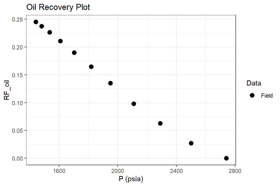
p3 <- mbal_results %>% ggplot(aes(`P (psia)`, `RF_oil`, color = "Field")) +
  geom_point(size = 3) +
  scale_color_manual(name="Data", values=c("Field" = "black")) +
  ggtitle("Oil Recovery Plot") +
  theme_bw()

p3
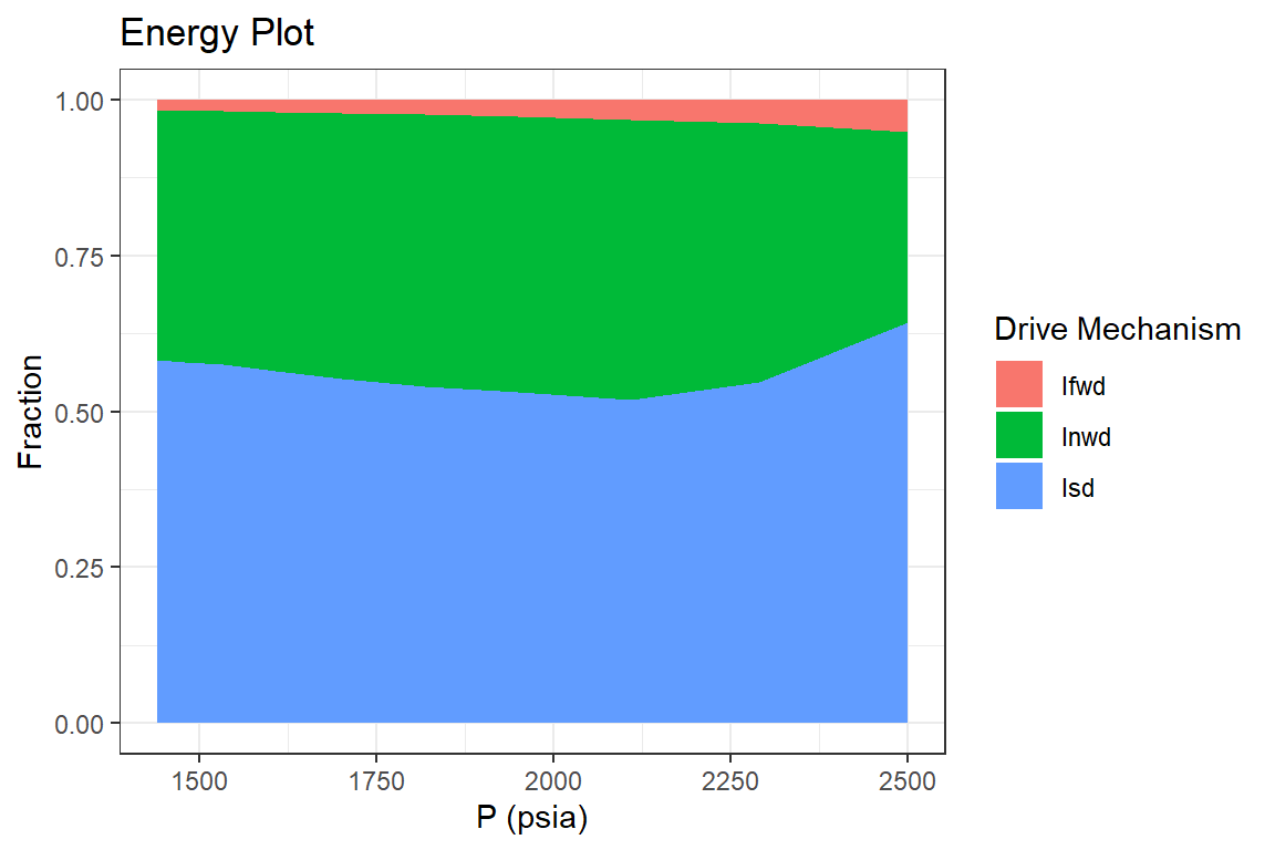
p4 <- mbal_results  %>%
  tidyr::pivot_longer(cols = c("Isd", "Inwd", "Ifwd"), names_to = "Drive Mechanism",
                      values_to = "Fraction", values_drop_na = TRUE) %>%
  ggplot(aes(`P (psia)`, Fraction, fill = `Drive Mechanism`)) +
  geom_area() +
  ggtitle("Energy Plot") +
  theme_bw()

p4
Example 6: Combination-Drive Black Oil Reservoir
Part I: History Match
library(Rmbal)
library(Rrelperm)
library(pracma)
library(ggplot2)
library(dplyr)
library(magrittr)

p_pvt <- c(2627, 2457, 2402, 2223, 2080, 1833, 1665, 1460, 1400)

Bo <- c(1.2681, 1.2554, 1.2512, 1.2383, 1.2278, 1.2074, 1.1949, 1.1802, 1.17)

Rs <- c(0.501, 0.4973, 0.4671, 0.4574, 0.4269, 0.4024, 0.3579, 0.3277, 0.2908) * 1e3

Bg <- c(1.0502, 1.0977, 1.1146, 1.2010, 1.2825, 1.4584, 1.6112, 1.8526, 2.1) / 1e3

Bw <- c(1.0228, 1.0232, 1.0233, 1.0237, 1.0240, 1.0246, 1.0250, 1.0254, 1.0258)

Rv <- rep(0, length(p_pvt))

muo <- rep(0.5, length(p_pvt))

muw <- rep(0.55, length(p_pvt))

mug <- rep(0.02, length(p_pvt))

pvt_table <- data.frame(p = p_pvt, Bo = Bo, Rs = Rs, Rv = Rv, Bg = Bg,
                               Bw = Bw, muo = muo, mug = mug, muw = muw)

p <- c(2627, 2457, 2402, 2223, 2080, 1833, 1665, 1460)

We <- rep(0, length.out = length(p))

Np <- c(0, 192821, 633942, 1314880, 1524400, 2152960, 2572000, 3200560)

Rp <- c(0, 490.1593, 492.2595, 540.4828, 558.2091, 629.7005, 708.8841, 853.8693)

Wp <- Wp <- c(0, 0, 0, 4, 7, 26, 60, 822)

Wi <- rep(0, length.out = length(p))

Gi <- rep(0, length.out = length(p))

wf <- c(1, 0, 1, 1, 1, 1, 1, 1)

mbal_optim_oil_lst <- mbal_optim_param_oil(input_unit = "Field", output_unit = "Field",
                                           unknown_param = "We",
                                           aquifer_model = "pot", N = 198e5,
                                           m = 0.05, phi = 0.28, swi = 0.25, Np = Np, Rp = Rp,
                                           Wp = Wp, Gi = Gi, Wi = Wi, We = NULL, pb = 2627,
                                           p = p, pvt = pvt_table, cf = 26e-6,
                                           phi_a = 0.28, perm_h_a = 100, h_a = 100,
                                           r_a = 2592.013, r_R = 1269.619, tetha = 360,
                                           muw_a = 0.55, cw_a = 2.28e-6, cf_a = 26e-6,
                                           wf = wf, sorw = 0.2, sorg = 0,
                                           mult_len = c(2))

time_lst <- mbal_time(c(0,305, 700, 1285, 1465, 2005, 2365, 2905), "day")

# a number of plots will be automatically generated for quality check

optim_results <- mbal_optim_oil(mbal_optim_oil_lst, time_lst)
glimpse(optim_results)
#> List of 18
#>  $ input_unit : chr "Field"
#>  $ output_unit: chr "Field"
#>  $ N          : num 19800000
#>  $ m          : num 0.05
#>  $ phi        : num 0.28
#>  $ swi        : num 0.25
#>  $ pb         : num 2627
#>  $ p          : num [1:8] 2627 2457 2402 2223 2080 ...
#>  $ cf         : num [1:8] 2.6e-05 2.6e-05 2.6e-05 2.6e-05 2.6e-05 2.6e-05 2.6e-05 2.6e-05
#>  $ pvt        :'data.frame': 9 obs. of  9 variables:
#>   ..$ p  : num [1:9] 2627 2457 2402 2223 2080 ...
#>   ..$ Bo : num [1:9] 1.27 1.26 1.25 1.24 1.23 ...
#>   ..$ Rs : num [1:9] 501 497 467 457 427 ...
#>   ..$ Rv : num [1:9] 0 0 0 0 0 0 0 0 0
#>   ..$ Bg : num [1:9] 0.00105 0.0011 0.00111 0.0012 0.00128 ...
#>   ..$ Bw : num [1:9] 1.02 1.02 1.02 1.02 1.02 ...
#>   ..$ muo: num [1:9] 0.5 0.5 0.5 0.5 0.5 0.5 0.5 0.5 0.5
#>   ..$ mug: num [1:9] 0.02 0.02 0.02 0.02 0.02 0.02 0.02 0.02 0.02
#>   ..$ muw: num [1:9] 0.55 0.55 0.55 0.55 0.55 0.55 0.55 0.55 0.55
#>  $ prod       :'data.frame': 8 obs. of  3 variables:
#>   ..$ Np: num [1:8] 0 192821 633942 1314880 1524400 ...
#>   ..$ Rp: num [1:8] 501 490 492 540 558 ...
#>   ..$ Wp: num [1:8] 0 0 0 4 7 26 60 822
#>  $ inj        :'data.frame': 8 obs. of  2 variables:
#>   ..$ Gi: num [1:8] 0 0 0 0 0 0 0 0
#>   ..$ Wi: num [1:8] 0 0 0 0 0 0 0 0
#>  $ We         : NULL
#>  $ aquifer    :List of 12
#>   ..$ input_unit : chr "Field"
#>   ..$ output_unit: chr "Field"
#>   ..$ model      : chr "pot"
#>   ..$ phi        : num 0.28
#>   ..$ h_a        : num 100
#>   ..$ r_a        : num 1532
#>   ..$ r_R        : num 1270
#>   ..$ tetha      : num 360
#>   ..$ c_water    : num 2.28e-06
#>   ..$ c_rock     : num 2.6e-05
#>   ..$ pressure   : num [1:8] 2627 2457 2402 2223 2080 ...
#>   ..$ mult_len   : num 1
#>   ..- attr(*, "class")= chr [1:2] "pot" "aquifer"
#>  $ wf         : num [1:8] 1 0 1 1 1 1 1 1
#>  $ sorw       : num 0.2
#>  $ sorg       : num 0
#>  $ p_est      : num [1:7] 2627 2379 2113 2058 1813 ...
#>  - attr(*, "class")= chr [1:2] "combination_oil" "mbal_oil"
Part II: Reservoir Performance
mbal_results <- mbal_perform_oil(optim_results, time_lst)

mbal_results
#>   P (psia) Eo (bbl/STB) Eg (bbl/SCF) Ew (bbl/STB) Ef (bbl/bbl) Eowf (bbl/STB)
#> 1     2627   0.00000000    0.0000000       0.0000     0.000000     0.00000000
#> 2     2402   0.02088494    0.0000644       0.0005     0.005850     0.03098276
#> 3     2223   0.02256360    0.0001508       0.0009     0.010504     0.04069571
#> 4     2080   0.05473325    0.0002323       0.0012     0.014222     0.07927574
#> 5     1833   0.08309824    0.0004082       0.0018     0.020644     0.11874701
#> 6     1665   0.15736272    0.0005610       0.0022     0.025012     0.20056222
#> 7     1460   0.23315558    0.0008024       0.0026     0.030342     0.28553235
#>   Egwf (bbl/SCF)  Et (bbl)   F (bbl)        We        Igd       Isd       Inwd
#> 1   0.000000e+00       0.0       0.0      0.00         NA        NA         NA
#> 2   7.276269e-05  773590.4  810965.7  73150.61 0.09951567 0.5345488 0.09455987
#> 3   1.658164e-04 1135335.5 1759421.9 131345.99 0.15877927 0.3935042 0.11568914
#> 4   2.526253e-04 2049480.4 2128380.4 177837.27 0.13549464 0.5287771 0.08677188
#> 5   4.377232e-04 3132563.1 3313206.1 258140.38 0.15577217 0.5252393 0.08240549
#> 6   5.967764e-04 4997222.2 4527824.7 312759.51 0.13419950 0.6235028 0.06258667
#> 7   8.457768e-04 7043155.1 6897989.7 379407.85 0.13618847 0.6554563 0.05386902
#>        Ifwd          Iawd Itot     RF_oil     RF_gas       SOo       SGo  SWo
#> 1        NA            NA   NA 0.00000000 0.00000000 0.7500000 0.0000000 0.25
#> 2 0.2713757  0.000000e+00    1 0.03054168 0.02678148 0.5402420 0.2097580 0.25
#> 3 0.3320310 -3.606687e-06    1 0.04285250 0.04125775 0.5188036 0.2311964 0.25
#> 4 0.2489599 -3.497472e-06    1 0.07413610 0.07371811 0.5113559 0.2386441 0.25
#> 5 0.2365916 -8.504091e-06    1 0.10280770 0.11532068 0.4909592 0.2590408 0.25
#> 6 0.1797234 -1.230684e-05    1 0.14336751 0.18103957 0.4786985 0.2713015 0.25
#> 7 0.1546059 -1.196735e-04    1 0.16506636 0.25107155 0.4619185 0.2880815 0.25
#>         SOT        SGT       SWT qo (STB/day) qg (SCF/day) qw (STB/day)
#> 1 0.7142857 0.03571429 0.2500000       0.0000          0.0  0.000000000
#> 2 0.5116513 0.23626772 0.2520810     905.6314     445805.7  0.000000000
#> 3 0.4883854 0.25787816 0.2537364    1163.9966     681377.9  0.006837607
#> 4 0.4787555 0.26618554 0.2550589    1164.0000     779244.0  0.016666667
#> 5 0.4546085 0.28804863 0.2573428    1164.0000     934789.0  0.035185185
#> 6 0.4392188 0.30188550 0.2588957    1164.0000    1298694.2  0.094444444
#> 7 0.4179878 0.32124277 0.2607695    1164.0000    1684463.0  1.411111111
#>           fg           fw GOR (SCF/STB)      krg/kro
#> 1 0.00000000 0.000000e+00      501.0000 0.0000000000
#> 2 0.02192139 0.000000e+00      492.2595 0.0008965083
#> 3 0.11729462 4.286600e-06      585.3779 0.0049649180
#> 4 0.31190606 8.216950e-06      669.4536 0.0101343884
#> 5 0.35721705 1.648782e-05      803.0833 0.0193591691
#> 6 0.57082184 2.986917e-05     1115.7167 0.0408735202
#> 7 0.66091802 3.567742e-04     1447.1332 0.0702884894

p1 <- mbal_results %>% ggplot(aes(`P (psia)`, SOo, color = "Field")) +
  geom_point(size = 3) +
  scale_color_manual(name="Data", values=c("Field" = "black")) +
  ggtitle("Oil Saturation Plot") +
  theme_bw()

p1
p2 <- mbal_results %>% ggplot(aes(`P (psia)`, `GOR (SCF/STB)`, color = "Field")) +
  geom_point(size = 3) +
  scale_color_manual(name="Data", values = c("Field" = "black")) +
  ggtitle("GOR Plot") +
  theme_bw()

p2
p3 <- mbal_results %>% ggplot(aes(`P (psia)`, `RF_oil`, color = "Field")) +
  geom_point(size = 3) +
  scale_color_manual(name="Data", values=c("Field" = "black")) +
  ggtitle("Oil Recovery Plot") +
  theme_bw()

p3
p4 <- mbal_results  %>%
  tidyr::pivot_longer(cols = c("Igd","Isd", "Inwd", "Ifwd"), names_to = "Drive Mechanism",
                      values_to = "Fraction", values_drop_na = TRUE) %>%
  ggplot(aes(`P (psia)`, Fraction, fill = `Drive Mechanism`)) +
  geom_area() +
  ggtitle("Energy Plot") +
  theme_bw()

p4
Example 7: Undersaturated Black Oil Reservoir (Walsh, Ansah, & Raghavan, 1994)
Part I: Reservoir Forecast
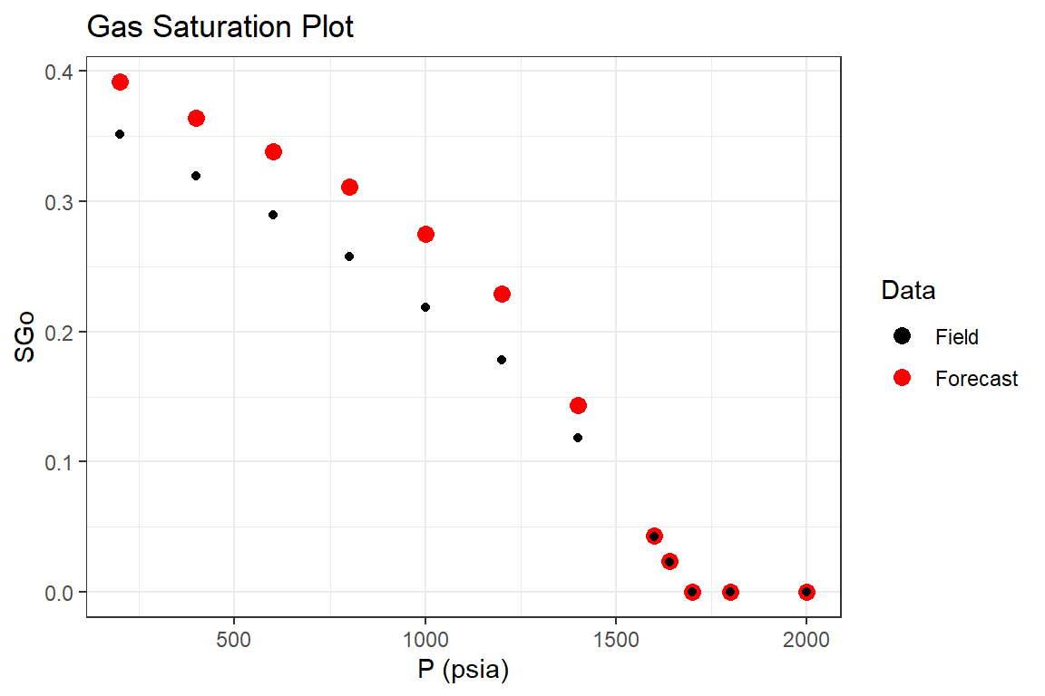
library(Rmbal)
library(Rrelperm)
library(pracma)
library(ggplot2)
library(dplyr)
library(magrittr)

p_pvt <- c(2000,    1800,   1700,   1640,   1600,   1400,   1200,   1000,   800, 600, 400, 200) # psia

Bo <- c(1.467, 1.472, 1.475, 1.463, 1.453, 1.408, 1.359, 1.322, 1.278, 1.237,
        1.194, 1.141) # RB/STB

Rs <- c(838.5, 838.5, 838.5, 816.1, 798.4, 713.4, 621, 548, 464, 383.9, 297.4,
        190.9) #SCF/STB

Bg <- c(1.749, 1.755, 1.758, 1.921, 1.977, 2.308, 2.73, 3.328, 4.163, 5.471,
        7.786, 13.331) / 1000 # RB/SCF

Rv <- c(1192.6, 1192.6, 1192.6, 0.2, 0.2,   0, 0, 0, 0, 0, 0, 0) / 1e6 # STB/SCF

cw <- 2e-6

Bwi <- 1.0

Bw <- Bwi * exp(cw * (p_pvt[1] - p_pvt))


muo <- c(0.3201,    0.3114, 0.3071, 0.3123, 0.316, 0.34,    0.371, 0.397, 0.432, 0.471,
         0.518, 0.589)  # cp

muw <- rep(0.25, length(p_pvt))

mug <- c(0.3201, 0.3114, 0.3071, 0.0157, 0.0155, 0.014, 0.0138, 0.0132, 0.0126, 0.0121,
         0.0116,    0.0108) # cp

pvt_table <- data.frame(p = p_pvt, Bo = Bo, Rs = Rs, Rv = Rv, Bg = Bg,
                               Bw = Bw, muo = muo, mug = mug, muw = muw)

p <- c(2000,    1800,   1700,   1640,   1600,   1400,   1200,   1000,   800, 600, 400, 200) # psia

Gi <- rep(0, length.out = length(p))

wf <- rep(1, length.out = length(p))

# generating a set of pseudo relative permeability curves using
# laboratory 'Kr' values

sg_lab <- c(0.05, 0.152, 0.248, 0.352, 0.448, 0.552, 0.65)

krg_lab <- c(0, 0.05, 0.09, 0.18, 0.3, 0.5, 1)

kro_lab <- c(1, 0.6, 0.35, 0.13, 0.04, 0.01, 0)

swcrit_lab <- 0.2

sgcrit_lab <- 0.05

sorgr_lab <- 0.15

fun_kr <- function(x, swcrit, sgcrit, sorg, sg, krg, kro) {

  kr_est <- Rrelperm::kr2p_gl(SWCON = swcrit, SOIRG = sorg, SORG = sorg,
                               SGCON = sgcrit, SGCRIT = sgcrit, KRGCL = 1,
                               KROGCG = 1, NG = x[1], NOG = x[2], NP = 101)

   krg_est_sub <- approx(x = kr_est[,1], y = kr_est[,3], xout = sg, rule = 2)$y

   kro_est_sub <- approx(x = kr_est[,1], y = kr_est[,4], xout = sg, rule = 2)$y

   error <- (krg - krg_est_sub) ^ 2 + (kro - kro_est_sub) ^ 2

   return(error)
}

par <- c(2, 2)

opt_results <- minpack.lm::nls.lm(par = par, fn = fun_kr, swcrit = swcrit_lab,
                                  sgcrit = sgcrit_lab, sorg = sorgr_lab, sg = sg_lab,
                                  krg = krg_lab, kro = kro_lab,
                                  lower = c(0.1,0.1), upper = c(10,10))

sol <- opt_results$par

sol
#> [1] 3.157478 2.740570

rel_perm <- as.data.frame(Rrelperm::kr2p_gl(SWCON = swcrit_lab, SOIRG = sorgr_lab,
                                            SORG = sorgr_lab, SGCON = sgcrit_lab,
                                            SGCRIT = sgcrit_lab, KRGCL = 1,
                                            KROGCG = 1, NG = sol[1], NOG = sol[2],
                                            NP = 101))

colnames(rel_perm) <- c("Sg", "Sl", "Krg", "Krog")

p_forecast <- p

Gi_forecast <- Gi

wf_forecast <- wf

time_lst_forecast <- mbal_time(c(1:length(p_forecast)), "year")


forecast_lst <- mbal_forecast_param_oil(input_unit = "Field", output_unit = "Field",
                                        N = 1e6, m = 0.0, phi = 0.1, swi = 0.2,
                                        Gi = Gi_forecast, pb = 1688, p = p_forecast, pvt = pvt_table,
                                        cf = 2e-6, wf = wf_forecast, sorg = 0.15, rel_perm = rel_perm)

forecast_results <- mbal_forecast_oil(forecast_lst, time_lst_forecast)

forecast_results
#>    P (psia)       SOo        SGo SWo       SOT           SGT SWT GOR (SCF/STB)
#> 1      2000 0.8000000 0.00000000 0.2 0.8000000 -5.551115e-17 0.2      838.5000
#> 2      1800 0.8000000 0.00000000 0.2 0.8000000 -5.551115e-17 0.2      838.5000
#> 3      1700 0.8000000 0.00000000 0.2 0.8000000 -5.551115e-17 0.2      838.5000
#> 4      1640 0.7760603 0.02393968 0.2 0.7760603  2.393968e-02 0.2      816.1000
#> 5      1600 0.7568933 0.04310670 0.2 0.7568933  4.310670e-02 0.2      798.4000
#> 6      1400 0.6567060 0.14329396 0.2 0.6567060  1.432940e-01 0.2      779.9858
#> 7      1200 0.5712189 0.22878111 0.2 0.5712189  2.287811e-01 0.2     1393.2373
#> 8      1000 0.5253609 0.27463906 0.2 0.5253609  2.746391e-01 0.2     2492.8351
#> 9       800 0.4892171 0.31078287 0.2 0.4892171  3.107829e-01 0.2     4082.2189
#> 10      600 0.4615355 0.33846451 0.2 0.4615355  3.384645e-01 0.2     5637.4153
#> 11      400 0.4361405 0.36385948 0.2 0.4361405  3.638595e-01 0.2     7032.5091
#> 12      200 0.4081428 0.39185717 0.2 0.4081428  3.918572e-01 0.2     8162.1692
#>         RF_oil      RF_gas Liq_volume Igd       Isd Inwd        Ifwd Iawd Itot
#> 1  0.000000000 0.000000000  1.0000000  NA        NA   NA          NA   NA   NA
#> 2  0.003994721 0.003994721  1.0000000   0 0.8503070    0 0.149693029    0    1
#> 3  0.006318892 0.006318892  1.0000000   0 0.8583354    0 0.141664611    0    1
#> 4  0.027267733 0.026987916  0.9714233   0 0.9609887    0 0.039011263    0    1
#> 5  0.044759320 0.043827610  0.9482533   0 0.9737390    0 0.026261005    0    1
#> 6  0.144719675 0.137909903  0.8298311   0 0.9886352    0 0.011364829    0    1
#> 7  0.229232788 0.247430386  0.6959327   0 0.9928034    0 0.007196600    0    1
#> 8  0.271270328 0.344842981  0.5775993   0 0.9946722    0 0.005327778    0    1
#> 9  0.298042320 0.449808570  0.4504689   0 0.9961593    0 0.003840732    0    1
#> 10 0.315811886 0.552798243  0.3321593   0 0.9972770    0 0.002722969    0    1
#> 11 0.330173640 0.661302918  0.2208247   0 0.9982155    0 0.001784493    0    1
#> 12 0.344056159 0.787087298  0.1167364   0 0.9990470    0 0.000952989    0    1

reservoir_performance_table <- data.frame(p = p)

reservoir_performance_table$`RF_oil` <- c(0, 0.4,   0.5, 2.7,   4.4, 11.3, 16.1,
                                          19.3, 22.2,   24.3,   26.2,   27.9) / 100

reservoir_performance_table$`Sg` <- c(0, 0, 0, 2.9, 5.3, 14.8, 22.3, 27.3, 32.2,
                                      36.2, 39.9,   43.9) * 0.8 / 100

reservoir_performance_table$`GOR` <- c(0.84,    0.84,   0.84,   0.82,   0.8,    1.41,   2.17,
                                       2.7, 3.52,   4.58,   5.56,   6.79) * 1000 # SCF/STB

p1 <- forecast_results %>% ggplot(aes(`P (psia)`, SGo, color = "Forecast")) +
  geom_point(size = 3) +
  geom_point(data = reservoir_performance_table, aes(`p`, Sg, color = "Field"))+
  scale_color_manual(name="Data", values=c("Forecast" = "red", "Field" = "black")) +
  ggtitle("Gas Saturation Plot") +
  theme_bw()

p1
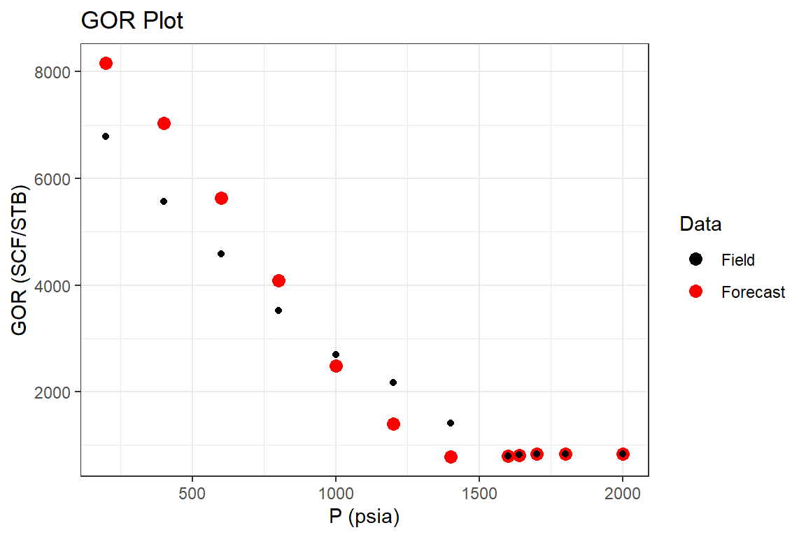
p2 <- forecast_results %>% ggplot(aes(`P (psia)`, `GOR (SCF/STB)`, color = "Forecast")) +
  geom_point(size = 3) +
  geom_point(data = reservoir_performance_table, aes(`p`, GOR, color = "Field"))+
  scale_color_manual(name="Data", values=c("Forecast" = "red", "Field" = "black")) +
  ggtitle("GOR Plot") +
  theme_bw()

p2
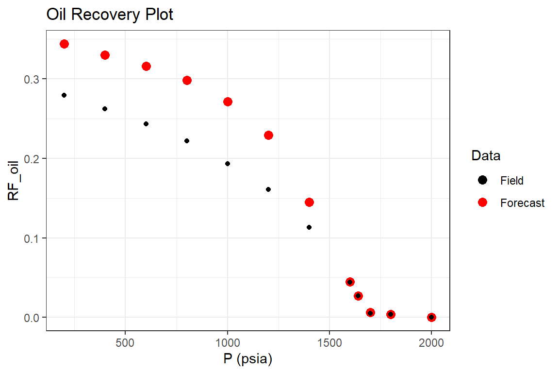
p3 <- forecast_results %>% ggplot(aes(`P (psia)`, `RF_oil`, color = "Forecast")) +
  geom_point(size = 3) +
  geom_point(data = reservoir_performance_table, aes(`p`, RF_oil, color = "Field"))+
  scale_color_manual(name="Data", values=c("Forecast" = "red", "Field" = "black")) +
  ggtitle("Oil Recovery Plot") +
  theme_bw()

p3
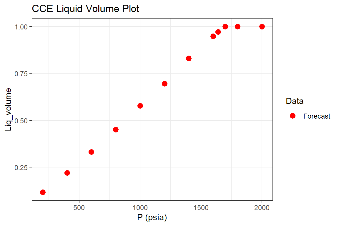
p4 <- forecast_results %>% ggplot(aes(`P (psia)`, `Liq_volume`, color = "Forecast")) +
  geom_point(size = 3) +
  scale_color_manual(name="Data", values=c("Forecast" = "red")) +
  ggtitle("CCE Liquid Volume Plot") +
  theme_bw()

p4
p5 <- forecast_results  %>%
  tidyr::pivot_longer(cols = c("Isd", "Ifwd"), names_to = "Drive Mechanism",
                      values_to = "Fraction", values_drop_na = TRUE) %>%
  ggplot(aes(`P (psia)`, Fraction, fill = `Drive Mechanism`)) +
  geom_area() +
  ggtitle("Energy Plot") +
  theme_bw()

p5
References
Ahmed, T., & McKinney, P. D. (2004). Advanced Reservoir Engineering (p. 424). Gulf Professional Publishing.
Dake, L. P. (1983). Fundamentals of Reservoir Engineering (p. 462). Elsevier Science.
Pletcher, J. L. (2002). Improvements to Reservoir Material-Balance Methods. SPE Reservoir Evaluation & Engineering, 5(01), 49–59. https://doi.org/10.2118/75354-PA
Walsh, M. P., Ansah, J., & Raghavan, R. (1994). New, generalized material balance as an equation of a straight line: Part 1- Applications to undersaturated, volumetric reservoirs. Proceedings of the Permian Basin Oil & Gas Recovery Conference, 549–564. https://doi.org/10.2118/27684-MS